8 Prepare genotypic data
-
Context and Purpose:
- Depending on whether parent- vs. mate-selection are intended, there are several formats to-be-constructed / computed from the downloaded genotypic data.
- Potentially, do exploratory / preliminary assessment of population structure, esp. any divergence between “training” samples and selection candidates (“test”).
Upstream: Section 7 - quality control steps for phenotype data
Downstream: All analyses relying on genotypic data
-
Inputs:
For parent selection: An imputed allele-dosage matrix downloaded from BreedBase (
data/BreedBaseGenotypesDownload.tsv)-
For mate selection:
An imputed variant call format (VCF) file downloaded from BreedBase (
data/BreedBaseGenotypesDownload.vcf)A centimorgan-scale genetic map with positions on the same reference genome version as the VCF. Can be sourced from the Cassavabase FTP, FTP archive, or another alternative.
-
Expected outputs:
For parent selection: a MAF filtered, dosage matrix, possibly with some samples removed relative to the database download.
-
For mate selection:
a haplotype matrix extracted from the VCF
a dosage matrix (computed from the haplotype matrix)
a filtered SNP list
Interpolated genetic map, a cM position for each SNP
For parent and mate selection: genomic relationship matrices (GRMs, aka kinship matrices), possibly both additive and dominance relationship matrices, constructed based on the dosage matrix.
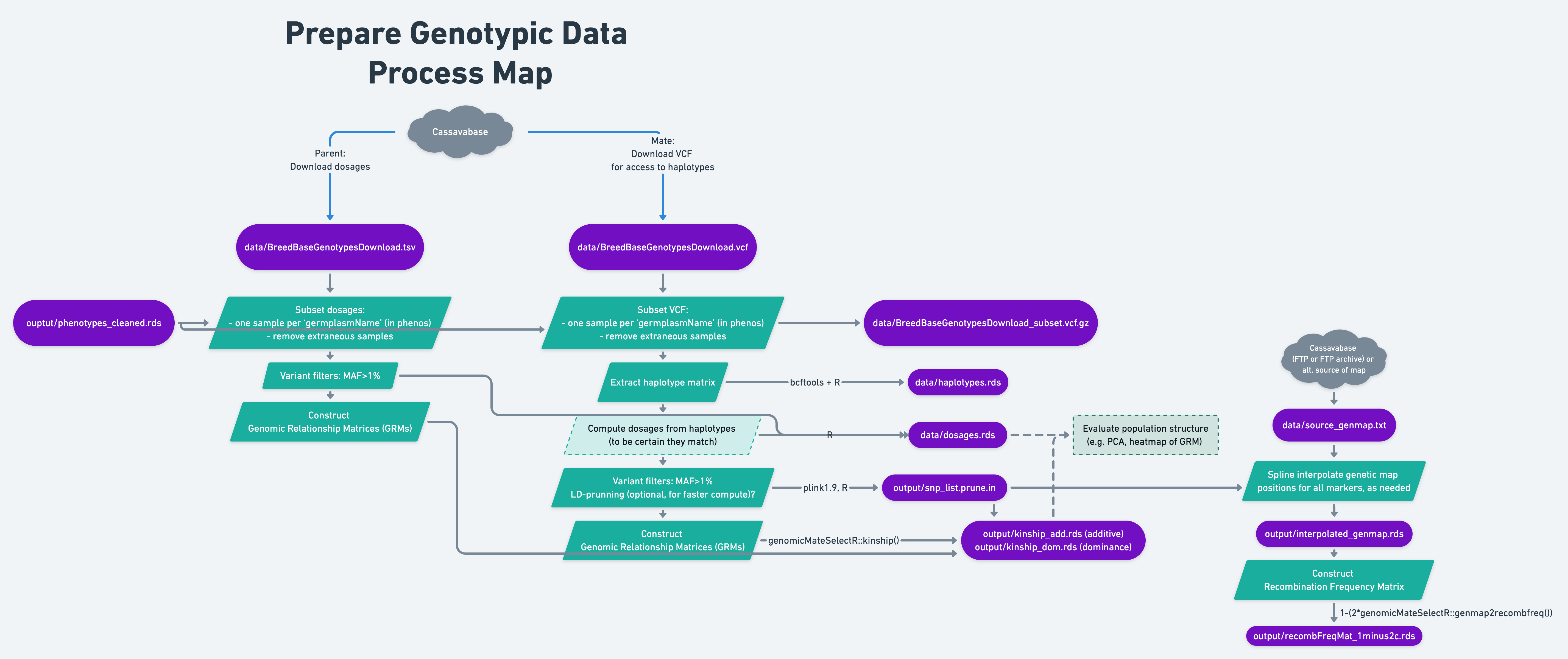
8.2 Parent vs. Mate Selection?
The following sections will exemplify the genomic mate selection as opposed to the somewhat simpler genomic parent selection pathway along the process map. This chapter can be simplified / mostly avoided if parent selection is sufficient.
8.5 Remote access the server
These steps will vary a bit depending on your system.
Instructions for BioHPC access are here: https://biohpc.cornell.edu/lab/doc/BioHPCLabexternal.pdf
First, remote login, using ssh
ssh userid@serverid.biohpc.cornell.edu
For example:
ssh mw489@cbsumm21.biohpc.cornell.eduInput your password when prompted.
pwdShould show something like /home/mw489/ (but your userid)
8.6 [INSTRUCTOR’S STEPs]
DON’T DO THESE STEPS, UNLESS YOU ARE ME, WHICH YOU ARE NOT ^_~!!
Create a sub-folder for analysis
I create a sub-folder for the analysis.
I created one with same name as my example GitHub repository for this workshop, like so:
mkdir GSexample2022;
cd GSexample2022;
mkdir data;
mkdir output;
Transfer data to CBSU
Now, on my local computer, navigate in the command line to data/
Use scp to transfer the VCF file downloaded from Cassavabase to the server.
Also copy the “cleaned_phenos.rds” from last week, which is in the output/:
scp BreedBaseGenotypesDownload.vcf mw489@cbsulogin.biohpc.cornell.edu:GSexample2022/data/
cd ../output;
scp phenotypes_cleaned.rds mw489@cbsulogin.biohpc.cornell.edu:GSexample2022/output/
Copy data to reserved servers /workdir/
mkdir /workdir/mw489/;Then I copy my GSexample2022 directory and its contents into that sub-folder.
cp -r ~/GSexample2022 /workdir/mw489/; 8.7 [EVERYONE’S STEPS]
8.7.1 Create a directory on /workdir/
Go to /workdir/
cd /workdir/Create a directory with your username:
Example:
mkdir youruserid/;Create a sub-directory for this analysis.
Example:
mkdir /workdir/youruserid/yourprojectnameNavigate into your subdirectory on /workdir/ (empty now).
Example:
cd /workdir/youruserid/yourprojectnameCopy the data/ and output/ from my /workdir/mw489/GSexample2022/ location, into yours.
Example:
cp -r /workdir/mw489/GSexample2022/data /workdir/youruserid/yourprojectname/
cp -r /workdir/mw489/GSexample2022/output /workdir/youruserid/yourprojectname/
Check that its there. Example:
ls /workdir/youruserid/yourprojectname/data/Now you should be ready to go.
Do all remaining steps within the directory you just created.
8.7.2 Install R packages to server
First time on the server and using R there?
Type R and then press “enter” to start R. (Later type q() + enter to quit R)…
Then install packages like so:
install.packages(c("tidyverse","workflowr", "sommer", "lme4", "devtools"))
devtools::install_github("wolfemd/genomicMateSelectR", ref = 'master')
If asked “do you want to install dependencies” and given a long list, type “1” + Enter to install ALL packages it asks. This will ensure you have everything you need.
8.8 Introducing VCF files
Some links:
- https://en.wikipedia.org/wiki/Variant_Call_Format
- Detailed specifications: https://samtools.github.io/hts-specs/VCFv4.2.pdf
- VCF poster: http://vcftools.sourceforge.net/VCF-poster.pdf
8.9 Check the VCF
Check the VCF ‘manually.’
- Are the number of samples and sites what you expected?
vcftools --vcf data/BreedBaseGenotypesDownload.vcf
# VCFtools - 0.1.16
# (C) Adam Auton and Anthony Marcketta 2009
#
# Parameters as interpreted:
#   --vcf data/BreedBaseGenotypesDownload.vcf
#
# After filtering, kept 1207 out of 1207 Individuals
# After filtering, kept 61239 out of a possible 61239 Sites
# Run Time = 16.00 seconds- Are the data phased?
- What FORMAT fields are present? At a minimum, should include GT field.
- Do the column-names after FORMAT (should be sample names) look right / make sense?
- Do the SNP IDs in the “ID” field make sense?
Let’s take a look at our VCF file:
# look at the header of the VCF file
# print the "top-left" corner of the file
cat data/BreedBaseGenotypesDownload.vcf | head -n50 | cut -c1-100
8.10 Subset VCF
- There may be multiple imputed DNA samples corresponding to a single unique ‘germplasmName.’ For matching to the phenotypic observations in downstream analyses, a single entry in the VCF file must be chosen per ‘germplasmName.’
- Remove extraneous samples, if any.
- For example / tutorial purposes ONLY: randomly sample and subset the number of SNPs to only a few thousand, for quick, local computations.
8.10.1 Remove duplicate samples
Cassavabase returned multiple columns in the VCF file with the same column-name, because of multiple tissue_samples per germplasmName. This prevents using certain tools, e.g. bcftools which errors.
Try this and you’ll see:
bcftools query --list-samples data/BreedBaseGenotypesDownload.vcfManual solution required:
Write just the column-names of the VCF to disk. Here’s a one-liner:
egrep "^#CHROM" data/BreedBaseGenotypesDownload.vcf | head -n1 > data/vcf_colnames.txtRead the column-names-file to R. Exclude the first 9 elements as they are standard VCF columns, not “germplasmName”
library(genomicMateSelectR) # to get the %>% loaded

vcf_sample_names<-readLines("data/vcf_colnames.txt") %>%
     strsplit(.,"\t") %>% unlist() %>%
     .[10:length(.)]
# Check how many sample names are duplicated?
table(duplicated(vcf_sample_names))
#>
#> FALSE  TRUE
#>   963   244
Quite a few duplicates.
Next, I (1) create unique names for each sample column in the VCF file, (2) write the “unique_names_for_vcf.txt” to disk and (3) use it to replace the current sample column names in the VCF. Finally, I (4) subset the VCF to only one unique instance of each name.
First, manipulate names using R.
# create unique names for each VCF
unique_names_for_vcf<-tibble(vcfName=vcf_sample_names) %>%
     # create an overall index to ensure I can recover the original column order
     mutate(vcfIndex=1:n()) %>%
     # now for each vcfName create an sub-index, to distinguish among duplicates
     group_by(vcfName) %>%
     # sub-index
     mutate(vcfNameIndex=1:n(),
            # For the first (or only) instance of each unique vcfName
            vcfName_Unique=ifelse(vcfNameIndex==1,
                                  # return the original name
                                  vcfName,
                                  # for all subsequent (duplicate) names,
                                  #put a unique-ified name by pasting the sub-index
                                  paste0(vcfName,".",vcfNameIndex)))
# Write the "unique_names_for_vcf.txt" to disk
write.table(unique_names_for_vcf$vcfName_Unique,file = "data/unique_names_for_vcf.txt",
            row.names = F, col.names = F, quote = F)
# Create also a list containing only one instance of each unique name, the first instance
subset_unique_names_for_vcf<-unique_names_for_vcf %>%
     filter(vcfNameIndex==1) %$%
     vcfName_Unique
# Write that list to disk for subsetting the VCF downstream
write.table(subset_unique_names_for_vcf,file = "data/subset_unique_names_for_vcf.txt",
            row.names = F, col.names = F, quote = F)
Now in the command line:
bcftools reheader to replace the sample names in the VCF with the unique ones.
# replace sample names in original VCF with unique ones (creates a new VCF)
bcftools reheader --samples data/unique_names_for_vcf.txt data/BreedBaseGenotypesDownload.vcf > data/BreedBaseGenotypesDownload_1.vcf;
# overwrite the original VCF with the new  that has unique names
mv data/BreedBaseGenotypesDownload_1.vcf data/BreedBaseGenotypesDownload.vcf;
# check that the names are now unique by printing sample list
bcftools query --list-samples data/BreedBaseGenotypesDownload.vcf
Now subset the VCF to only a single instance of each “germplasmName” with vcftools.
vcftools --vcf data/BreedBaseGenotypesDownload.vcf --keep data/subset_unique_names_for_vcf.txt --recode --stdout | bgzip -c > data/BreedBaseGenotypes_subset.vcf.gz
# uses stdout and bgzip to output a gzipped vcf file; saves disk space!
vcftools --gzvcf data/BreedBaseGenotypes_subset.vcf.gz
#VCFtools - 0.1.16
#(C) Adam Auton and Anthony Marcketta 2009
# Parameters as interpreted:
# --gzvcf data/BreedBaseGenotypes_subset.vcf.gz
#
# Using zlib version: 1.2.11
# After filtering, kept 963 out of 963 Individuals
# After filtering, kept 61239 out of a possible 61239 Sites
# Run Time = 2.00 seconds8.10.2 Check genotype-to-phenotype matches
- Do the number of unique germplasmName (in the “cleaned phenos” from the previous step) matching samples in the VCF make sense? Are there as many as expected? If not, you will need to figure out why not.
phenos<-readRDS(here::here("output","phenotypes_cleaned.rds"))

# vector of the unique germplasmName in the field trial data
germplasm_with_phenos<-unique(phenos$germplasmName)
length(germplasm_with_phenos)
#> [1] 1002
How many matches to the VCF?
subset_unique_names_for_vcf<-read.table(file = "data/subset_unique_names_for_vcf.txt",
                                        stringsAsFactors = F)$V1

table(germplasm_with_phenos %in% subset_unique_names_for_vcf)
#>
#> FALSE  TRUE
#>   652   350
350 matches. Does that make sense? Yes. We ended up excluding the “genetic gain” trial from the phenotypes b/c actually there were no trait scores.
To be sure, I look at the names of: (1) the genotyped and phenotyped, (2) the genotyped but not phenotyped, (3) the phenotyped but not genotyped.
# geno and pheno
subset_unique_names_for_vcf[subset_unique_names_for_vcf %in% germplasm_with_phenos]
# pheno not geno
germplasm_with_phenos[!germplasm_with_phenos %in% subset_unique_names_for_vcf]
# geno not pheno
subset_unique_names_for_vcf[!subset_unique_names_for_vcf %in% germplasm_with_phenos]
To diagnose some the phenotyped-but-not-genotyped, I actually resorted to searching a few on Cassavabase to verify that there were non-genotyped lines in the trials I downloaded.
For the genotyped-but-not-phenotyped, indeed the names are all “genetic gain” population clones.
Probably the details above will change if I go back and choose better example trials.
The checklist and approach to verifying it all should stay the same.
8.10.3 Subset SNPs (for tutorial purposes)
For example / tutorial purposes ONLY: randomly sample and subset the number of SNPs to only a few thousand, for quick, local computations.
# write the positions list
# first two columns (chrom. and position) of the VCF
# ignoring the header rows
cat data/BreedBaseGenotypesDownload.vcf | grep -v "^#" | cut -f1-2 > data/BreedBaseGenotypesDownload.positions
Read into R, sample 4000 at random
library(genomicMateSelectR)
set.seed(1234)
read.table(here::here("data","BreedBaseGenotypesDownload.positions"),
           header = F, stringsAsFactors = F) %>%
     dplyr::slice_sample(n=4000) %>%
     arrange(V1,V2) %>%
     write.table(.,file = "data/BreedBaseGenotypes_subset.positions",
                 row.names = F, col.names = F, quote = F)
Subset the VCF using the randomly sampled list of positions.
vcftools --vcf data/BreedBaseGenotypesDownload.vcf \
--keep data/subset_unique_names_for_vcf.txt \
--positions data/BreedBaseGenotypes_subset.positions \
--recode --stdout | bgzip -c > data/BreedBaseGenotypes_subset.vcf.gz
# VCFtools - 0.1.16
# (C) Adam Auton and Anthony Marcketta 2009
#
# Parameters as interpreted:
#   --vcf data/BreedBaseGenotypesDownload.vcf
#   --keep data/subset_unique_names_for_vcf.txt
#   --positions data/BreedBaseGenotypes_subset.positions
#   --recode
#   --stdout
#
# Keeping individuals in 'keep' list
# After filtering, kept 963 out of 1207 Individuals
# Outputting VCF file...
# After filtering, kept 4000 out of a possible 61239 Sites
# Run Time = 8.00 seconds
vcftools --gzvcf data/BreedBaseGenotypes_subset.vcf.gz8.10.4 LD-prunning SNPs (for computational savings)
NOT DEMONSTRATED HERE, YET. In practice, when predicting cross-variances, it can still be very computationally intensive with large numbers of markers. Previously, I used plink --indep-pairwise to prune markers based on linkage disequilibrium. I found an LD-prunned subset that had similar accuracy to the full set, but less than half the markers. Subsequently, I used the full set to predict cross means, but the LD-pruned marker subset for the cross variances predictions of >250K crosses of 719 candidate parents in IITA’s 2021 crossing block.
8.11 Haplotype matrix from VCF
Extract haplotypes from VCF with bcftools convert --hapsample
bcftools convert --hapsample data/BreedBaseGenotypes_subset data/BreedBaseGenotypes_subset.vcf.gz
# Hap file: data/BreedBaseGenotypes_subset.hap.gz
# Sample file: data/BreedBaseGenotypes_subset.samples
# [W::vcf_parse_format] FORMAT 'NT' at 1:652699 is not defined in the header, assuming Type=String
# 4000 records written, 0 skipped: 0/0/0 no-ALT/non-biallelic/filtered
Read haps to R and format them.
library(genomicMateSelectR)
library(data.table)
#>
#> Attaching package: 'data.table'
#> The following objects are masked from 'package:dplyr':
#>
#>     between, first, last
#> The following object is masked from 'package:purrr':
#>
#>     transpose
vcfName<-"BreedBaseGenotypes_subset"
haps<-fread(paste0("data/",vcfName,".hap.gz"),
            stringsAsFactors = F,header = F) %>%
  as.data.frame
sampleids<-fread(paste0("data/",vcfName,".samples"),
                 stringsAsFactors = F,header = F,skip = 2) %>%
  as.data.frame
Add sample ID’s.
hapids<-sampleids %>%
     select(V1,V2) %>%
     mutate(SampleIndex=1:nrow(.)) %>%
     rename(HapA=V1,HapB=V2) %>%
     pivot_longer(cols=c(HapA,HapB),
                  names_to = "Haplo",values_to = "SampleID") %>%
     mutate(HapID=paste0(SampleID,"_",Haplo)) %>%
     arrange(SampleIndex)
colnames(haps)<-c("Chr","HAP_ID","Pos","REF","ALT",hapids$HapID)
dim(haps)
#> [1] 4000 1931
Format, transpose, convert to matrix.
8.12 Dosage matrix from haps
To ensure consistency in allele counting, create dosage from haps manually.
The counted allele in the dosage matrix, which will be used downstream to construct kinship matrices and estimate marker effects, should be the ALT allele. This will ensure a match to the haplotype matrix, where a “1” indicates the presence of the ALT allele.
The BreedBase system currently (as of Jan. 2022) gives dosages that count the REF allele and we need to fix this.
Here’s my tidyverse-based approach, using group_by() plus summarise() to sum the two haplotypes for each individual across all loci.
dosages<-haps %>%
     as.data.frame(.) %>%
     rownames_to_column(var = "GID") %>%
     separate(GID,c("SampleID","Haplo"),"_Hap",remove = T) %>%
     select(-Haplo) %>%
     group_by(SampleID) %>%
     summarise(across(everything(),~sum(.))) %>%
     ungroup() %>%
     column_to_rownames(var = "SampleID") %>%
     as.matrix %>%
     # preserve same order as in haps
     .[sampleids$V1,]
dim(dosages)
#> [1]  963 4000

dosages[1:5,1:5]
#>                    1_652699_G_C 1_868970_G_T 1_943129_T_A
#> IITA-TMS-IBA30572             1            0            0
#> IITA-TMS-IBA940237            0            0            1
#> IITA-TMS-IBA961642            1            1            0
#> IITA-TMS-ONN920168            0            0            0
#> IITA-TMS-WAR4080              1            0            0
#>                    1_1132830_A_T 1_1310706_A_T
#> IITA-TMS-IBA30572              1             0
#> IITA-TMS-IBA940237             1             1
#> IITA-TMS-IBA961642             2             0
#> IITA-TMS-ONN920168             0             0
#> IITA-TMS-WAR4080               1             0
haps[1:10,1:5]
#>                         1_652699_G_C 1_868970_G_T
#> IITA-TMS-IBA30572_HapA             1            0
#> IITA-TMS-IBA30572_HapB             0            0
#> IITA-TMS-IBA940237_HapA            0            0
#> IITA-TMS-IBA940237_HapB            0            0
#> IITA-TMS-IBA961642_HapA            1            0
#> IITA-TMS-IBA961642_HapB            0            1
#> IITA-TMS-ONN920168_HapA            0            0
#> IITA-TMS-ONN920168_HapB            0            0
#> IITA-TMS-WAR4080_HapA              0            0
#> IITA-TMS-WAR4080_HapB              1            0
#>                         1_943129_T_A 1_1132830_A_T
#> IITA-TMS-IBA30572_HapA             0             1
#> IITA-TMS-IBA30572_HapB             0             0
#> IITA-TMS-IBA940237_HapA            0             0
#> IITA-TMS-IBA940237_HapB            1             1
#> IITA-TMS-IBA961642_HapA            0             1
#> IITA-TMS-IBA961642_HapB            0             1
#> IITA-TMS-ONN920168_HapA            0             0
#> IITA-TMS-ONN920168_HapB            0             0
#> IITA-TMS-WAR4080_HapA              0             0
#> IITA-TMS-WAR4080_HapB              0             1
#>                         1_1310706_A_T
#> IITA-TMS-IBA30572_HapA              0
#> IITA-TMS-IBA30572_HapB              0
#> IITA-TMS-IBA940237_HapA             0
#> IITA-TMS-IBA940237_HapB             1
#> IITA-TMS-IBA961642_HapA             0
#> IITA-TMS-IBA961642_HapB             0
#> IITA-TMS-ONN920168_HapA             0
#> IITA-TMS-ONN920168_HapB             0
#> IITA-TMS-WAR4080_HapA               0
#> IITA-TMS-WAR4080_HapB               0
8.13 Variant filters
In this case, simple: keep only positions with >1% minor allele frequency.
# use function built into genomicMateSelectR
dosages<-maf_filter(dosages,thresh = 0.01)
dim(dosages)
#> [1]  963 3986
# subset haps to match
haps<-haps[,colnames(dosages)]8.14 Genomic Relationship Matrices (GRMs)
In the example below, I use the genomicMateSelectR function kinship() to construct additive (A) and dominance (D) relationship matrices.
A<-kinship(dosages,type="add")
D<-kinship(dosages,type="domGenotypic")
saveRDS(A,file=here::here("output","kinship_add.rds"))
saveRDS(D,file=here::here("output","kinship_dom.rds"))
For more information on the models to-be-implemented downstream, see this vignette for genomicMateSelectR, the references cited therein.
8.15 Recombination Frequency Matrix
Matrix needed for cross-variance predictions.
8.15.1 Source a genetic map
- Must match the reference genome of the marker set to be used in prediction
- Not necessarily the exact markerset, but overlap is ideal
I source a single genome-wide file representing the ICGMC concensus genetic map on the V6 Cassava Reference genome. The file is on the Cassavabase FTP-archive, here.
genmap<-read.table("https://cassavabase.org/ftp/marnin_datasets/NGC_BigData/CassavaGeneticMap/cassava_cM_pred.v6.allchr.txt",
                   header = F, sep=';', stringsAsFactors = F) %>%
     rename(SNP_ID=V1,Pos=V2,cM=V3) %>%
  as_tibble
genmap %>% dim
#> [1] 120979      3
120K positions.
genmap %>% head
#> # A tibble: 6 × 3
#>   SNP_ID     Pos    cM
#>   <chr>    <int> <dbl>
#> 1 S1_26576 26576   2.7
#> 2 S1_26624 26624   2.7
#> 3 S1_26659 26659   2.7
#> 4 S1_27720 27720   2.7
#> 5 S1_27739 27739   2.7
#> 6 S1_27746 27746   2.7
snps_genmap<-tibble(DoseSNP_ID=colnames(dosages)) %>%
     separate(DoseSNP_ID,c("Chr","Pos","Ref","Alt"),remove = F) %>%
     mutate(SNP_ID=paste0("S",Chr,"_",Pos)) %>%
     full_join(genmap %>%
                    separate(SNP_ID,c("Chr","POS"),"_",remove = F) %>%
                    select(-POS) %>%
                    mutate(Chr=gsub("S","",Chr)) %>%
                    mutate(across(everything(),as.character)))
#> Joining, by = c("Chr", "Pos", "SNP_ID")
snps_genmap %>%
  ggplot(.,aes(x=as.integer(Pos)/1000/1000,y=as.numeric(cM))) +
  geom_point() +
  theme_bw() +
  facet_wrap(~as.integer(Chr))
#> Warning: Removed 1567 rows containing missing values
#> (geom_point).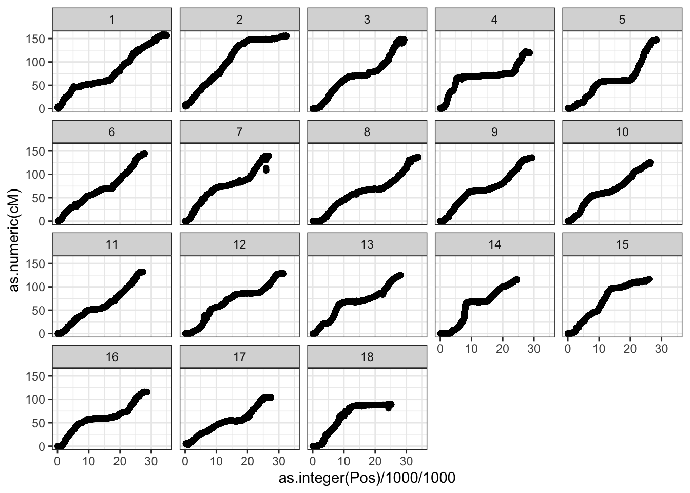
8.15.2 Interpolate genetic map
interpolate_genmap<-function(data){
  # for each chromosome map
  # find and _decrements_ in the genetic map distance
  # fix them to the cumulative max to force map to be only increasing
  # fit a spline for each chromosome
  # Use it to predict values for positions not previously on the map
  # fix them AGAIN (in case) to the cumulative max, forcing map to only increase
  data_forspline<-data %>%
    filter(!is.na(cM)) %>%
    mutate(cumMax=cummax(cM),
           cumIncrement=cM-cumMax) %>%
    filter(cumIncrement>=0) %>%
    select(-cumMax,-cumIncrement)

  spline<-data_forspline %$% smooth.spline(x=Pos,y=cM,spar = 0.75)

  splinemap<-predict(spline,x = data$Pos) %>%
    as_tibble(.) %>%
    rename(Pos=x,cM=y) %>%
    mutate(cumMax=cummax(cM),
           cumIncrement=cM-cumMax) %>%
    mutate(cM=cumMax) %>%
    select(-cumMax,-cumIncrement)

  return(splinemap)
}
splined_snps_genmap<-snps_genmap %>%
  select(-cM) %>%
  mutate(Pos=as.numeric(Pos)) %>%
  left_join(snps_genmap %>%
              mutate(across(c(Pos,cM),as.numeric)) %>%
              arrange(Chr,Pos) %>%
              nest(-Chr) %>%
              mutate(data=map(data,interpolate_genmap)) %>%
              unnest(data)) %>%
  distinct
#> Warning: All elements of `...` must be named.
#> Did you want `data = c(DoseSNP_ID, Pos, Ref, Alt, SNP_ID, cM)`?
#> Joining, by = c("Chr", "Pos")
splined_snps_genmap %>%
     filter(DoseSNP_ID %in% colnames(dosages)) %>%
     mutate(Map="Spline") %>%
     bind_rows(snps_genmap %>%
                    filter(DoseSNP_ID %in% colnames(dosages),
                           !is.na(cM)) %>%
                    mutate(across(c(Pos,cM),as.numeric)) %>%
                    arrange(Chr,Pos) %>% mutate(Map="Data")) %>%
  ggplot(.,aes(x=Pos/1000/1000,y=cM,color=Map, shape=Map),alpha=0.3,size=0.75) +
  geom_point() +
  theme_bw() + facet_wrap(~as.integer(Chr), scales='free_x')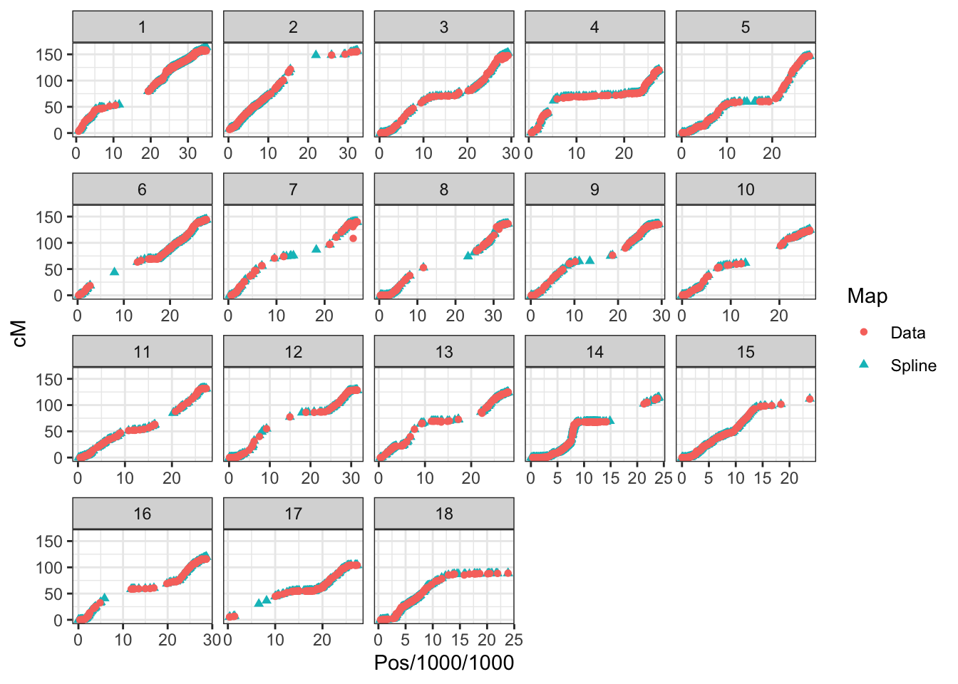
Save the interpolated map, just for the marker loci to-be-used downstream.
8.15.3 Recomb. freq. matrix
genmap<-readRDS(file=here::here("output","interpolated_genmap.rds"))
m<-genmap$cM;
names(m)<-genmap$DoseSNP_ID
recombFreqMat<-1-(2*genmap2recombfreq(m,nChr = 18))
saveRDS(recombFreqMat,file=here::here("output","recombFreqMat_1minus2c.rds"))
See also, genomicMateSelectR vignette.
8.16 Copy files back to your computer
Option 1) FileZilla
Option 2) Command line:
On my local computer, on your command line.
Navigate to the project directory containing the data/ and output/ directories.
scp mw489@cbsumm21.biohpc.cornell.edu:/workdir/youruserid/yourprojectname/data/BreedBaseGenotypes_subset.vcf.gz data/
scp mw489@cbsumm21.biohpc.cornell.edu:/workdir/youruserid/yourprojectname/data/dosages.rds data/
scp mw489@cbsumm21.biohpc.cornell.edu:/workdir/youruserid/yourprojectname/data/haplotypes.rds data/
scp mw489@cbsumm21.biohpc.cornell.edu:/workdir/youruserid/yourprojectname/output/kinship_add.rds output/
scp mw489@cbsumm21.biohpc.cornell.edu:/workdir/youruserid/yourprojectname/output/kinship_dom.rds output/
scp mw489@cbsumm21.biohpc.cornell.edu:/workdir/youruserid/yourprojectname/output/recombFreqMat_1minus2c.rds output/
scp mw489@cbsumm21.biohpc.cornell.edu:/workdir/youruserid/yourprojectname/output/interpolated_genmap.rds output/
Option 3) I’ll provide Google Drive links to download the big files, and post the small ones to my GitHub repo