Results

workflowr

• Summary
• Checks
• Past versions

Last updated: 2021-09-18

Checks: 7 0

Knit directory: IITA_2021GS/

This reproducible R Markdown analysis was created with workflowr (version 1.6.2). The Checks tab describes the reproducibility checks that were applied when the results were created. The Past versions tab lists the development history.

---

R Markdown file: up-to-date

Great! Since the R Markdown file has been committed to the Git repository, you know the exact version of the code that produced these results.

Environment: empty

Great job! The global environment was empty. Objects defined in the global environment can affect the analysis in your R Markdown file in unknown ways. For reproduciblity it’s best to always run the code in an empty environment.

Seed: set.seed(20210504)

The command set.seed(20210504) was run prior to running the code in the R Markdown file. Setting a seed ensures that any results that rely on randomness, e.g. subsampling or permutations, are reproducible.

Session information: recorded

Great job! Recording the operating system, R version, and package versions is critical for reproducibility.

Cache: none

Nice! There were no cached chunks for this analysis, so you can be confident that you successfully produced the results during this run.

File paths: relative

Great job! Using relative paths to the files within your workflowr project makes it easier to run your code on other machines.

Repository version: 01fb4d2

Great! You are using Git for version control. Tracking code development and connecting the code version to the results is critical for reproducibility.

The results in this page were generated with repository version 01fb4d2. See the Past versions tab to see a history of the changes made to the R Markdown and HTML files.

Note that you need to be careful to ensure that all relevant files for the analysis have been committed to Git prior to generating the results (you can use wflow_publish or wflow_git_commit). workflowr only checks the R Markdown file, but you know if there are other scripts or data files that it depends on. Below is the status of the Git repository when the results were generated:

Ignored files:
    Ignored:    .DS_Store
    Ignored:    .Rhistory
    Ignored:    .Rproj.user/
    Ignored:    analysis/.DS_Store
    Ignored:    code/.DS_Store
    Ignored:    data/.DS_Store

Untracked files:
    Untracked:  data/DatabaseDownload_2021Aug08/
    Untracked:  data/DatabaseDownload_2021May04/
    Untracked:  data/GBSdataMasterList_31818.csv
    Untracked:  data/IITA_GBStoPhenoMaster_33018.csv
    Untracked:  data/Mate_selection_parental.pool.xlsx
    Untracked:  data/NRCRI_GBStoPhenoMaster_40318.csv
    Untracked:  data/PedigreeGeneticGainCycleTime_aafolabi_01122020.xls
    Untracked:  data/Report-DCas21-6038/
    Untracked:  data/blups_forGP.rds
    Untracked:  data/chr1_RefPanelAndGSprogeny_ReadyForGP_72719.fam
    Untracked:  data/dosages_IITA_2021Aug09.rds
    Untracked:  data/haps_IITA_2021Aug09.rds
    Untracked:  data/recombFreqMat_1minus2c_2021Aug02.qs
    Untracked:  output/

Unstaged changes:
    Modified:   analysis/inputsForSimulationV2.Rmd

Note that any generated files, e.g. HTML, png, CSS, etc., are not included in this status report because it is ok for generated content to have uncommitted changes.

---

These are the previous versions of the repository in which changes were made to the R Markdown (analysis/07-Results.Rmd) and HTML (docs/07-Results.html) files. If you’ve configured a remote Git repository (see ?wflow_git_remote), click on the hyperlinks in the table below to view the files as they were in that past version.

File	Version	Author	Date	Message
Rmd	01fb4d2	wolfemd	2021-09-18	Updated mate predictions and results page - predicted >250K crosses of 719 parents at Ubiaja now.
html	ceae21a	wolfemd	2021-08-26	Build site.
html	19c3a38	wolfemd	2021-08-19	Build site.
html	e029efc	wolfemd	2021-08-12	Build site.
Rmd	efebeab	wolfemd	2021-08-12	Cross-validation and genomic mate predictions complete. All results updated.
html	f0a71e4	wolfemd	2021-08-11	Build site.
Rmd	ab2c1ec	wolfemd	2021-08-11	workflowr::wflow_publish(files = “analysis/07-Results.Rmd”)
html	934141c	wolfemd	2021-07-14	Build site.
html	cc1eb4b	wolfemd	2021-07-14	Build site.
Rmd	772750a	wolfemd	2021-07-14	DirDom model and selection index calc fully integrated functions.

---

The summaries below correspond to the results of analyses outlined here and linked in the navbar above.

1. Preliminary summaries of the population, the data, results of pedigree validation,
2. Prediction accuracy estimates
3. Genomic Predictions and Genomic mate selection.

Preliminary summaries

Raw data

Summary of the number of unique plots, locations, years, etc. in the cleaned plot-basis data (output/IITA_ExptDesignsDetected_2021May10.rds, download from FTP). See the data cleaning step here for details.

library(tidyverse); library(magrittr); library(ragg)
rawdata<-readRDS(file=here::here("output","IITA_ExptDesignsDetected_2021Aug08.rds"))
rawdata %>% 
  summarise(Nplots=nrow(.),
            across(c(locationName,studyYear,studyName,TrialType,GID), ~length(unique(.)),.names = "N_{.col}")) %>% 
  rmarkdown::paged_table()

This is not the same number of clones as are expected to be genotyped-and-phenotyped.

Next, a break down of the plots based on the trial design and TrialType (really a grouping of the population that is breeding program specific), captured by two logical variables, CompleteBlocks and IncompleteBlocks.

rawdata %>% 
  count(TrialType,CompleteBlocks,IncompleteBlocks) %>% 
  spread(TrialType,n) %>% 
  rmarkdown::paged_table()

Next, look at breakdown of plots by TrialType (rows) and locations (columns):

rawdata %>% 
  count(locationName,TrialType) %>% 
  spread(locationName,n) %>% 
  rmarkdown::paged_table()

traits<-c("MCMDS","DM","PLTHT","BRNHT1","BRLVLS","HI",
          "logDYLD", # <-- logDYLD now included. 
          "logFYLD","logTOPYLD","logRTNO","TCHART","LCHROMO","ACHROMO","BCHROMO")
rawdata %>% 
  select(locationName,studyYear,studyName,TrialType,any_of(traits)) %>% 
  pivot_longer(cols = any_of(traits), values_to = "Value", names_to = "Trait") %>% 
  ggplot(.,aes(x=Value,fill=Trait)) + geom_histogram() + facet_wrap(~Trait, scales='free') + 
  theme_bw() + scale_fill_viridis_d() + 
  labs(title = "Distribution of Raw Phenotypic Values")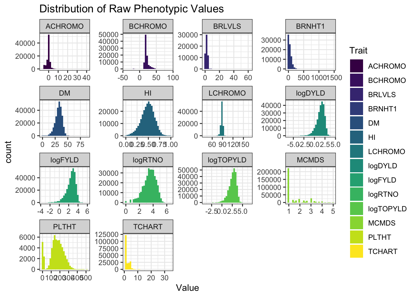

Past versions of unnamed-chunk-4-1.png

Version	Author	Date
f0a71e4	wolfemd	2021-08-11
cc1eb4b	wolfemd	2021-07-14

How many genotyped-and-phenotyped clones?

genotypedAndPhenotypedClones<-rawdata %>% 
  select(locationName,studyYear,studyName,TrialType,germplasmName,FullSampleName,GID,any_of(traits)) %>% 
  pivot_longer(cols = any_of(traits), values_to = "Value", names_to = "Trait") %>%
  filter(!is.na(Value),!is.na(FullSampleName)) %>%
  distinct(germplasmName,FullSampleName,GID)

There are 8962 genotyped-and-phenotyped clones!

genotypedAndPhenotypedClones %>% 
  rmarkdown::paged_table()

BLUPs

Summarize the BLUPs from the training data, leveraging for each clone data across trials/locations without genomic information and to be used as input for genomic prediction downstream (data/blups_forCrossVal.rds, download from FTP). See the mixed-model analysis step here and a subsequent processing step here for details.

blups<-readRDS(file=here::here("data","blups_forGP.rds")) 
gidWithBLUPs<-blups %>% select(Trait,blups) %>% unnest(blups) %$% unique(GID)
rawdata %>% 
  select(observationUnitDbId,GID,any_of(blups$Trait)) %>% 
  pivot_longer(cols = any_of(blups$Trait), 
               names_to = "Trait", 
               values_to = "Value",values_drop_na = T) %>% 
  filter(GID %in% gidWithBLUPs) %>% 
  group_by(Trait) %>% 
  summarize(Nplots=n()) %>% 
  ungroup() %>% 
  left_join(blups %>% 
              mutate(Nclones=map_dbl(blups,~nrow(.)),
                     avgREL=map_dbl(blups,~mean(.$REL)),
                     Vg=map_dbl(varcomp,~.["GID!GID.var","component"]),
                     Ve=map_dbl(varcomp,~.["R!variance","component"]),
                     H2=Vg/(Vg+Ve)) %>% 
              select(-blups,-varcomp)) %>% 
  mutate(across(is.numeric,~round(.,3))) %>% arrange(desc(H2)) %>% 
  rmarkdown::paged_table()

• Nplots, Nclones: the number of unique plots and clones per trait
• avgREL: the mean reliability of BLUPs, where for the jth clone, \(REL_j = 1 - \frac{PEV_j}{V_g}\)
• Vg, Ve, H2: the genetic and residual variance components and the broad sense heritability (\(H^2=\frac{V_g}{V_g+V_e}\)).

blups %>% 
  select(Trait,blups) %>% 
  unnest(blups) %>% 
  ggplot(.,aes(x=drgBLUP,fill=Trait)) + geom_histogram() + facet_wrap(~Trait, scales='free') + 
  theme_bw() + scale_fill_viridis_d() + theme(legend.position = 'none') + 
  labs(title = "Distribution of de-regressed BLUP Values")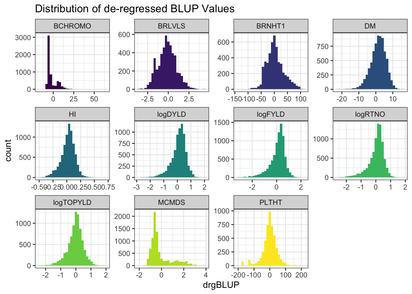

Past versions of unnamed-chunk-8-1.png

Version	Author	Date
f0a71e4	wolfemd	2021-08-11
cc1eb4b	wolfemd	2021-07-14

• de-regressed BLUPs or \(drgBLUP_j = \frac{BLUP_j}{REL_j}\)

blups %>% 
  select(Trait,blups) %>% 
  unnest(blups) %>% 
  ggplot(.,aes(x=Trait,y=REL,fill=Trait)) + geom_boxplot(notch=T) + #facet_wrap(~Trait, scales='free') + 
  theme_bw() + scale_fill_viridis_d() + 
  theme(axis.text.x = element_text(angle=90),
        legend.position = 'none') + 
  labs(title = "Distribution of BLUP Reliabilities")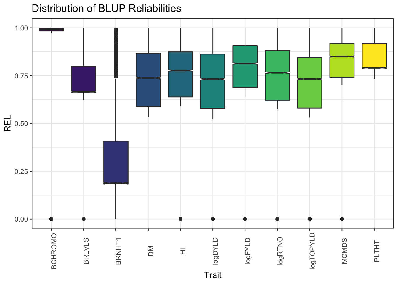

Past versions of unnamed-chunk-9-1.png

Version	Author	Date
f0a71e4	wolfemd	2021-08-11
cc1eb4b	wolfemd	2021-07-14

Marker density and distribution

Summarize the marker data (data/dosages_IITA_filtered_2021May13.rds, download from FTP). See the pre-processing steps here.

library(tidyverse); library(magrittr);
snps<-readRDS(file=here::here("data","dosages_IITA_2021Aug09.rds"))
mrks<-colnames(snps) %>% 
  tibble(SNP_ID=.) %>% 
  separate(SNP_ID,c("Chr","Pos","Allele"),"_") %>% 
  mutate(Chr=as.integer(gsub("S","",Chr)),
         Pos=as.numeric(Pos))
rm(snps);
mrks %>% 
  ggplot(.,aes(x=Pos,fill=as.character(Chr))) + geom_histogram() + 
  facet_wrap(~Chr,scales = 'free') + theme_bw() + 
  scale_fill_viridis_d() + theme(legend.position = 'none',
                                 axis.text.x = element_text(angle=90))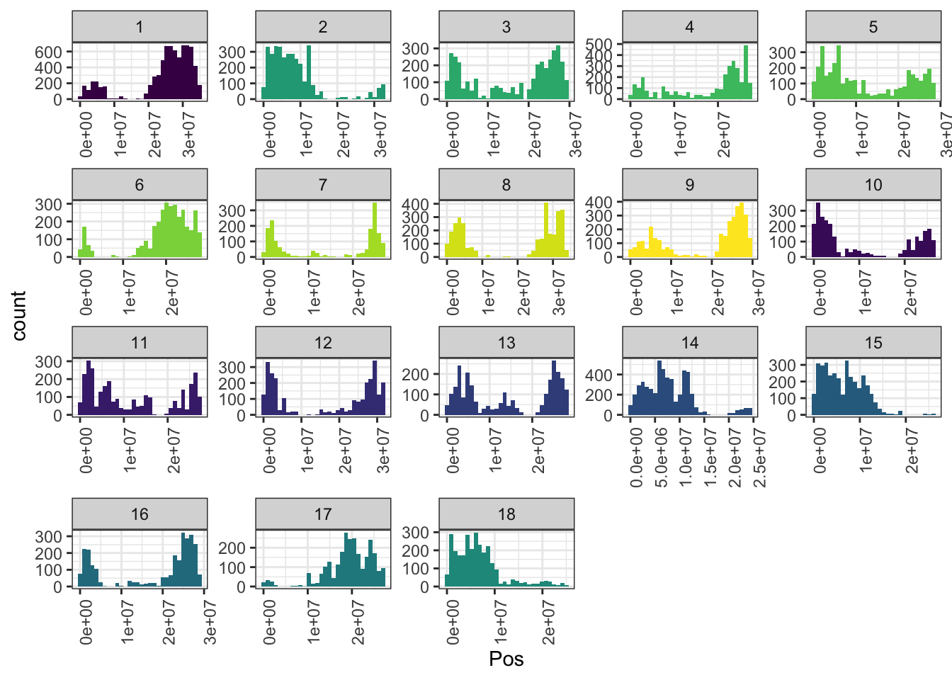

Past versions of unnamed-chunk-10-1.png

Version	Author	Date
f0a71e4	wolfemd	2021-08-11

In total, 61239 SNPs genome-wide. Broken down by chromosome:

mrks %>% count(Chr,name = "Nsnps") %>% rmarkdown::paged_table()

Pedigree validation

Introduced new downstream procedures (the parent-wise cross-validation, which rely on a trusted pedigree. To support this, introduced a new pedigree-validation step. The pedigree and validation results are summarized below.

The verified pedigree (output/verified_ped.txt), can be downloaded from the FTP here).

library(tidyverse); library(magrittr);
ped2check_genome<-readRDS(file=here::here("output","ped2check_genome.rds"))
ped2check_genome %<>% 
  select(IID1,IID2,Z0,Z1,Z2,PI_HAT)
ped2check<-read.table(file=here::here("output","ped2genos.txt"),
                      header = F, stringsAsFactors = F) %>% 
  rename(FullSampleName=V1,DamID=V2,SireID=V3)
ped2check %<>% 
  select(FullSampleName,DamID,SireID) %>% 
  inner_join(ped2check_genome %>% 
               rename(FullSampleName=IID1,DamID=IID2) %>% 
               bind_rows(ped2check_genome %>% 
                           rename(FullSampleName=IID2,DamID=IID1))) %>% 
  distinct %>% 
  mutate(FemaleParent=case_when(Z0<0.32 & Z1>0.67~"Confirm",
                                       SireID==DamID & PI_HAT>0.6 & Z0<0.3 & Z2>0.32~"Confirm",
                                       TRUE~"Reject")) %>% 
  select(-Z0,-Z1,-Z2,-PI_HAT) %>% 
  inner_join(ped2check_genome %>% 
               rename(FullSampleName=IID1,SireID=IID2) %>% 
               bind_rows(ped2check_genome %>% 
                           rename(FullSampleName=IID2,SireID=IID1))) %>% 
  distinct %>% 
  mutate(MaleParent=case_when(Z0<0.32 & Z1>0.67~"Confirm",
                                       SireID==DamID & PI_HAT>0.6 & Z0<0.3 & Z2>0.32~"Confirm",
                                       TRUE~"Reject")) %>% 
  select(-Z0,-Z1,-Z2,-PI_HAT)
rm(ped2check_genome)

ped2check %<>% 
  mutate(Cohort=NA,
         Cohort=ifelse(grepl("TMS20",FullSampleName,ignore.case = T),"TMS20",
                       ifelse(grepl("TMS19",FullSampleName,ignore.case = T),"TMS19",
                              ifelse(grepl("TMS18",FullSampleName,ignore.case = T),"TMS18",
                                     ifelse(grepl("TMS17",FullSampleName,ignore.case = T),"TMS17",
                                            ifelse(grepl("TMS16",FullSampleName,ignore.case = T),"TMS16",
                                                   ifelse(grepl("TMS15",FullSampleName,ignore.case = T),"TMS15",
                                                          ifelse(grepl("TMS14",FullSampleName,ignore.case = T),"TMS14",
                                                                 ifelse(grepl("TMS13|2013_",FullSampleName,ignore.case = T),"TMS13","GGetc")))))))))

Proportion of accessions with male, female or both parents in pedigree confirm-vs-rejected?

ped2check %>% 
  count(FemaleParent,MaleParent) %>% 
  mutate(Prop=round(n/sum(n),2))

  FemaleParent MaleParent    n Prop
1      Confirm    Confirm 4473 0.72
2      Confirm     Reject  715 0.12
3       Reject    Confirm  442 0.07
4       Reject     Reject  576 0.09

Proportion of accessions within each Cohort with pedigree records confirmed-vs-rejected?

ped2check %>% 
  count(Cohort,FemaleParent,MaleParent) %>% 
  spread(Cohort,n) %>% 
  mutate(across(is.numeric,~round(./sum(.),2))) %>% 
  rmarkdown::paged_table()

Use only fully-confirmed families / trios. Remove any without both parents confirmed.

ped<-read.table(here::here("output","verified_ped.txt"),
                header = T, stringsAsFactors = F) %>% 
  mutate(Cohort=NA,
         Cohort=ifelse(grepl("TMS20",FullSampleName,ignore.case = T),"TMS20",
                       ifelse(grepl("TMS19",FullSampleName,ignore.case = T),"TMS19",
                              ifelse(grepl("TMS18",FullSampleName,ignore.case = T),"TMS18",
                                     ifelse(grepl("TMS17",FullSampleName,ignore.case = T),"TMS17",
                                            ifelse(grepl("TMS16",FullSampleName,ignore.case = T),"TMS16",
                                                   ifelse(grepl("TMS15",FullSampleName,ignore.case = T),"TMS15",
                                                          ifelse(grepl("TMS14",FullSampleName,ignore.case = T),"TMS14",
                                                                 ifelse(grepl("TMS13|2013_",FullSampleName,ignore.case = T),"TMS13","GGetc")))))))))

Summary of family sizes

ped %>% 
  count(SireID,DamID) %$% summary(n)

   Min. 1st Qu.  Median    Mean 3rd Qu.    Max. 
   1.00    1.00    3.00    5.55    7.00   77.00 

ped %>% nrow(.) # 4473 pedigree entries

[1] 4473

ped %>% 
  count(Cohort,name = "Number of Verified Pedigree Entries")

  Cohort Number of Verified Pedigree Entries
1  GGetc                                  20
2  TMS13                                1786
3  TMS14                                1303
4  TMS15                                 589
5  TMS17                                  11
6  TMS18                                 592
7  TMS19                                  40
8  TMS20                                 132

ped %>% distinct(SireID,DamID) %>% nrow(.)

[1] 806

ped %>% 
  distinct(Cohort,SireID,DamID) %>% 
  count(Cohort,name = "Number of Families per Cohort")

  Cohort Number of Families per Cohort
1  GGetc                            18
2  TMS13                           119
3  TMS14                           234
4  TMS15                           198
5  TMS17                            10
6  TMS18                           172
7  TMS19                            30
8  TMS20                            28

806 families. Mean size 5.55, range 1-77.

Prediction accuracy estimates

Two cross-validation procedures were used to measure prediction accuracy.

First, a brand new procedure to assess the accuracy of genomic predictions of cross means and variances, which is called (parent-wise cross-validation.

Second, I also ran the standard 5 reps of 5-fold cross-validation, which measures the accuracy of predicting individual performance.

Both using a additive-plus-dominance model including a directional-dominance term (modelType="DirDom").

Here are the Selection index weights (provided by IITA) and used to compute the SELIND accuracy displayed further below.

# SELECTION INDEX WEIGHTS
## from IYR+IK
## note that not ALL predicted traits are on index
c(logFYLD=20,
  HI=10,
  DM=15,
  MCMDS=-10,
  logRTNO=12,
  logDYLD=20,
  logTOPYLD=15,
  PLTHT=10)

  logFYLD        HI        DM     MCMDS   logRTNO   logDYLD logTOPYLD     PLTHT 
       20        10        15       -10        12        20        15        10 

Plot SELIND prediction accuracy

library(ggdist)
# PARENT-WISE CV RESULTS
accuracy_full<-readRDS(here::here("output","parentWiseCV_full_set_CrossPredAccuracy.rds"))
accuracy_medium<-readRDS(here::here("output","parentWiseCV_medium_set_CrossPredAccuracy.rds"))
accuracy_reduced<-readRDS(here::here("output","parentWiseCV_reduced_set_CrossPredAccuracy.rds"))
accuracy<-accuracy_medium$meanPredAccuracy %>%
  filter(Trait=="SELIND") %>%
  mutate(VarComp=gsub("Mean","",predOf),
         predOf="Mean",
         Filter="LDprunedR2pt8 \n (~13K)") %>%
  bind_rows(accuracy_medium$varPredAccuracy %>%
              filter(Trait1=="SELIND") %>%
              rename(Trait=Trait1) %>%
              select(-Trait2) %>%
              mutate(VarComp=gsub("Var","",predOf),
                     predOf="Var",
                     Filter="LDprunedR2pt8 \n (~13K)")) %>%
  bind_rows(accuracy_reduced$meanPredAccuracy %>%
  filter(Trait=="SELIND") %>%
  mutate(VarComp=gsub("Mean","",predOf),
         predOf="Mean",
         Filter="LDprunedR2pt6 \n (~8K)") %>%
  bind_rows(accuracy_reduced$varPredAccuracy %>%
              filter(Trait1=="SELIND") %>%
              rename(Trait=Trait1) %>%
              select(-Trait2) %>%
              mutate(VarComp=gsub("Var","",predOf),
                     predOf="Var",
                     Filter="LDprunedR2pt6 \n (~8K)"))) %>%
    bind_rows(accuracy_full$meanPredAccuracy %>%
  filter(Trait=="SELIND") %>%
  mutate(VarComp=gsub("Mean","",predOf),
         predOf="Mean",
         Filter="FullSet \n (~33K)") %>%
  bind_rows(accuracy_full$varPredAccuracy %>%
              filter(Trait1=="SELIND") %>%
              rename(Trait=Trait1) %>%
              select(-Trait2) %>%
              mutate(VarComp=gsub("Var","",predOf),
                     predOf="Var",
                     Filter="FullSet \n (~33K)")))

recalculated_accuracy<-accuracy %>% 
  select(-AccuracyEst) %>% 
  unnest(predVSobs) %>% 
  select(-obsVar,-obsMean,-obsVar) %>% 
  mutate(predValue=ifelse(predOf=="Mean",predMean,predVar)) %>% 
  select(-predVar,-predMean) %>% 
  left_join(accuracy %>% 
              select(-AccuracyEst) %>% 
              filter(grepl("FullSet",Filter)) %>% 
              unnest(predVSobs) %>% 
              select(-predVar,-predMean) %>% 
              mutate(obsValue=ifelse(predOf=="Mean",obsMean,obsVar)) %>% 
              select(-obsMean,-obsVar,-Filter)) %>% 
  nest(predVSobs=c(sireID,damID,predValue,obsValue,famSize)) %>% 
  mutate(AccuracyEst=map_dbl(predVSobs,function(predVSobs){
    out<-psych::cor.wt(predVSobs[,c("predValue","obsValue")],
                       w = predVSobs$famSize) %$% r[1,2] %>%
      round(.,3)
    return(out) })) %>% 
  select(-predVSobs)   

# STANDARD CV RESULTS
standardCV_full<-readRDS(here::here("output",
                                    "standardCV_full_set_ClonePredAccuracy.rds"))
standardCV_medium<-readRDS(here::here("output",
                                    "standardCV_medium_set_ClonePredAccuracy.rds"))
standardCV_reduced<-readRDS(here::here("output",
                                       "standardCV_reduced_set_ClonePredAccuracy.rds"))
accuracy<-standardCV_full %>% 
  unnest(accuracyEstOut) %>% 
  select(-splits,-predVSobs,-seeds) %>% 
  filter(Trait=="SELIND") %>% 
  rename(Repeat=repeats,Fold=id,VarComp=predOf,AccuracyEst=Accuracy) %>% 
  mutate(Repeat=paste0("Repeat",Repeat),
         VarComp=gsub("GE","",VarComp),
         predOf="IndivPerformance",
         Filter="FullSet \n (~33K)") %>% 
    bind_rows(standardCV_medium %>% 
              unnest(accuracyEstOut) %>% 
              select(-splits,-predVSobs,-seeds) %>% 
              filter(Trait=="SELIND") %>% 
              rename(Repeat=repeats,Fold=id,VarComp=predOf,AccuracyEst=Accuracy) %>% 
              mutate(Repeat=paste0("Repeat",Repeat),
                     VarComp=gsub("GE","",VarComp),
                     predOf="IndivPerformance",
                    Filter="LDprunedR2pt8 \n (~13K)")) %>% 
  bind_rows(standardCV_reduced %>% 
              unnest(accuracyEstOut) %>% 
              select(-splits,-predVSobs,-seeds) %>% 
              filter(Trait=="SELIND") %>% 
              rename(Repeat=repeats,Fold=id,VarComp=predOf,AccuracyEst=Accuracy) %>% 
              mutate(Repeat=paste0("Repeat",Repeat),
                     VarComp=gsub("GE","",VarComp),
                     predOf="IndivPerformance",
                    Filter="LDprunedR2pt6 \n (~8K)")) %>% 
  bind_rows(recalculated_accuracy %>%
              mutate(predOf=paste0("Cross",predOf))) %>%
  mutate(Filter=factor(Filter,levels=c("FullSet \n (~33K)","LDprunedR2pt8 \n (~13K)","LDprunedR2pt6 \n (~8K)")),
         predOf=factor(predOf,levels=c("IndivPerformance","CrossMean","CrossVar")),
         VarComp=factor(VarComp,levels=c("BV","TGV"))) %>% droplevels

colors<-viridis::viridis(4)[1:2]

The figure below shows the ultimate summary of all cross-validation, the estimated accuracy predicting individual performance (clone means), cross-means and cross-variances on the selection index. Results from 5 repeats of 5-fold clone-wise (“standard”) and parent-wise (“NEW”) cross-validation are combined in this plot. See further below for a break down by trait. For the “CrossMean” and “CrossVar” panels, the y-axis “AccuracyEst” is the family-size weighted correlation between the predicted and observed cross means and variances. To fairly compare cross mean and variance accuracy across SNP sets, the observed means and variances from the full SNP set were used as the validation data for all sets. For the “IndivPerformance” panels, the y-axis is an un-weighted correlation between GBLUPs (i.e. GEBV/GETGV) and phenotypic (i.e. non-genomic or i.i.d. BLUPs). Predictions of breeding value (BV) and total genetic value (TGV) are distinguished in all plots and relate to the value of a cross for producing future parents and/or elite varieties, respectively among their offspring. Predictions of BV use only allele substitution effects (\(\alpha\)). Predictions of TGV incorporate dominance effects/variance. The modelType=DirDom was used.

Two SNP sets, one LD-pruned more than the other (reduced_set and full_set) were tested.

1. lightly LD-pruned: plink --indep-pairwise 50 25 0.98 (considered the “full_set”)
2. more strongly pruned plink --indep-pairwise 1000 'kb' 50 0.6 (considered the “reduced_set”)

accuracy %>% 
  ggplot(.,aes(x=VarComp,y=AccuracyEst,fill=VarComp)) +
  ggdist::stat_halfeye(adjust=0.5,.width = 0,fill='gray',width=0.75) +  
  geom_boxplot(width=0.12,notch = TRUE) +
  ggdist::stat_dots(side = "left",justification = 1.1,dotsize=0.6)+
  theme_bw() + 
  scale_fill_manual(values = colors) + 
  geom_hline(data = accuracy %>% distinct(predOf) %>% mutate(yint=c(NA,NA,0)),
             aes(yintercept = yint), color='black', size=0.9) +
  theme(axis.text.x = element_blank(),
        axis.title.x = element_blank(),
        strip.background = element_blank(),
        panel.grid.major = element_blank(),
        panel.grid.minor = element_blank(),
        axis.title = element_text(face='bold',color = 'black'),
        strip.text.x = element_text(face='bold',color='black',size=12),
        axis.text.y = element_text(face = 'bold',color='black'),
        legend.text = element_text(face='bold'),
        legend.position = 'bottom') +
  facet_grid(predOf~Filter,scales = 'free') + 
  labs(title="Accuracy predicting performance on the Selection Index",
       subtitle="Predictions of clone and cross performance (cross means and variances)")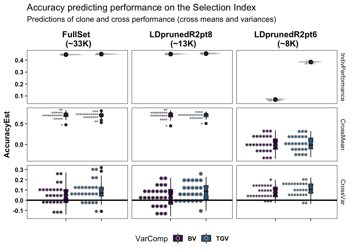 

Past versions of unnamed-chunk-22-1.png

Version	Author	Date
e029efc	wolfemd	2021-08-12
f0a71e4	wolfemd	2021-08-11

Based on the preliminary results (variance predictions not even done yet), the reduced_set (LDprunedR2pt6) suffers reduced prediction accuracy. I added a medium_set (LDprunedR2pt8) with about 13K SNP which produces GEBV/GETGV that are highly correlated with the full 33K SNP set and has the same accuracy.

Prediction accuracy estimates are in output/ (here) with filenames ending _ClonePredAccuracy.rds and _CrossPredAccuracy.rds.

For details on the cross-validation scheme, see the article (and for even more, the corresponding supplemental documentation here). See also the genomicMateSelectR::runParentWiseCrossVal() details section.

Plots with breakdowns by traits

Standard cross-validation

Results, broken down by trait, for the “standard” 5 repeats of 5-fold cross-validation on the accuracy predicting individual-level performance. Contrast to the cross-mean and cross-variance predictions newly implemented and plotted further below. c(“FullSet (~33K)”,“LDprunedR2pt8 (~13K)”,“LDprunedR2pt6 (~8K)”)

standardCV_full %>% 
  unnest(accuracyEstOut) %>% 
  select(-splits,-predVSobs,-seeds) %>% 
  mutate(Filter="Full") %>% 
  bind_rows(standardCV_medium %>% 
              unnest(accuracyEstOut) %>% 
              select(-splits,-predVSobs,-seeds) %>% 
              mutate(Filter="Medium")) %>% 
  mutate(Trait=factor(Trait,levels=c("SELIND",blups$Trait)),
         predOf=factor(paste0(predOf,"_",Filter),levels=c("GEBV_Full","GETGV_Full","GEBV_Medium","GETGV_Medium"))) %>% 
  ggplot(.,aes(x=predOf,y=Accuracy,fill=predOf,color=predOf)) + 
  geom_boxplot(notch = TRUE, color='gray40') +
  scale_fill_manual(values = viridis::viridis(4)[1:4]) + 
  scale_color_manual(values = viridis::viridis(4)[1:4]) + 
  #geom_hline(yintercept = 0, color='black', size=0.8) +
  facet_grid(.~Trait) + 
  labs(title="Accuracy predicting the performance of untested clones",
       subtitle="Standard 5-fold cross-validation") + 
  theme_bw() + 
  theme(axis.text.x = element_blank(),
        axis.title.x = element_blank(),
        strip.background = element_blank(),
        panel.grid.major = element_blank(),
        panel.grid.minor = element_blank(),
        legend.position='bottom',
        axis.text.y = element_text(face='bold'),
        axis.title.y = element_text(face='bold'),
        strip.text.x = element_text(face='bold'),
        plot.title = element_text(face='bold'),
        legend.title = element_text(face='bold'),
        legend.text = element_text(face='bold'),
        panel.spacing = unit(0.2, "lines"))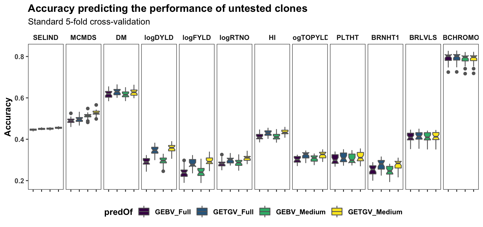

Past versions of unnamed-chunk-23-1.png

Version	Author	Date
e029efc	wolfemd	2021-08-12
f0a71e4	wolfemd	2021-08-11
cc1eb4b	wolfemd	2021-07-14

Parent-wise cross-validation

accuracy<-accuracy_medium$meanPredAccuracy %>%
  mutate(VarComp=gsub("Mean","",predOf),
         predOf="Mean",
         Filter="13K",
         Trait2=Trait) %>%
  rename(Trait1=Trait) %>% 
  bind_rows(accuracy_medium$varPredAccuracy %>%
              mutate(VarComp=gsub("Var","",predOf),
                     predOf="Var",
                     Filter="13K")) %>% 
bind_rows(accuracy_reduced$meanPredAccuracy %>%
  mutate(VarComp=gsub("Mean","",predOf),
         predOf="Mean",
         Filter="8K",
         Trait2=Trait) %>%
  rename(Trait1=Trait) %>% 
  bind_rows(accuracy_reduced$varPredAccuracy %>%
              mutate(VarComp=gsub("Var","",predOf),
                     predOf="Var",
                     Filter="8K"))) %>%
    bind_rows(accuracy_full$meanPredAccuracy %>%
  mutate(VarComp=gsub("Mean","",predOf),
         predOf="Mean",
         Filter="33K",
         Trait2=Trait) %>%
  rename(Trait1=Trait) %>% 
  bind_rows(accuracy_full$varPredAccuracy %>%
              mutate(VarComp=gsub("Var","",predOf),
                     predOf="Var",
                     Filter="33K")))

recalculated_accuracy<-accuracy %>% 
  select(-AccuracyEst) %>% 
  unnest(predVSobs) %>% 
  select(-obsVar,-obsMean,-obsVar) %>% 
  mutate(predValue=ifelse(predOf=="Mean",predMean,predVar)) %>% 
  select(-predVar,-predMean) %>% 
  left_join(accuracy %>% 
              select(-AccuracyEst) %>% 
              filter(grepl("33K",Filter)) %>% 
              unnest(predVSobs) %>% 
              select(-predVar,-predMean) %>% 
              mutate(obsValue=ifelse(predOf=="Mean",obsMean,obsVar)) %>% 
              select(-obsMean,-obsVar,-Filter)) %>% 
  nest(predVSobs=c(sireID,damID,predValue,obsValue,famSize)) %>% 
  mutate(AccuracyEst=map_dbl(predVSobs,function(predVSobs){
    out<-psych::cor.wt(predVSobs[,c("predValue","obsValue")],
                       w = predVSobs$famSize) %$% r[1,2] %>%
      round(.,3)
    return(out) })) %>% 
  select(-predVSobs)   

Cross-mean prediction accuracy

recalculated_accuracy %>% 
  filter(predOf=="Mean") %>% 
  mutate(Trait1=factor(Trait1,levels=c("SELIND",blups$Trait)),
         predOf=factor(paste0("Mean",VarComp,"_",Filter),
                       levels=c("MeanBV_33K","MeanTGV_33K","MeanBV_13K","MeanTGV_13K","MeanBV_8K","MeanTGV_8K"))) %>% 
  ggplot(.,aes(x=predOf,y=AccuracyEst,fill=predOf,color=Filter)) + 
  geom_boxplot(notch = TRUE, color='gray40') +
  scale_fill_manual(values = viridis::viridis(6)) + 
  scale_color_manual(values = viridis::viridis(6)) + 
  geom_hline(yintercept = 0, color='black', size=0.8) +
  facet_grid(.~Trait1) + 
  labs(title="Accuracy predicting the mean performance of offspring from untested crosses",
       subtitle="5-fold 'parent-wise' cross-validation") + 
  theme_bw() + 
  theme(axis.text.x = element_blank(),
        axis.title.x = element_blank(),
        strip.background = element_blank(),
        panel.grid.major = element_blank(),
        panel.grid.minor = element_blank(),
        legend.position='bottom',
        axis.text.y = element_text(face='bold'),
        axis.title.y = element_text(face='bold'),
        strip.text.x = element_text(face='bold'),
        plot.title = element_text(face='bold'),
        legend.title = element_text(face='bold'),
        legend.text = element_text(face='bold'),
        panel.spacing = unit(0.2, "lines"))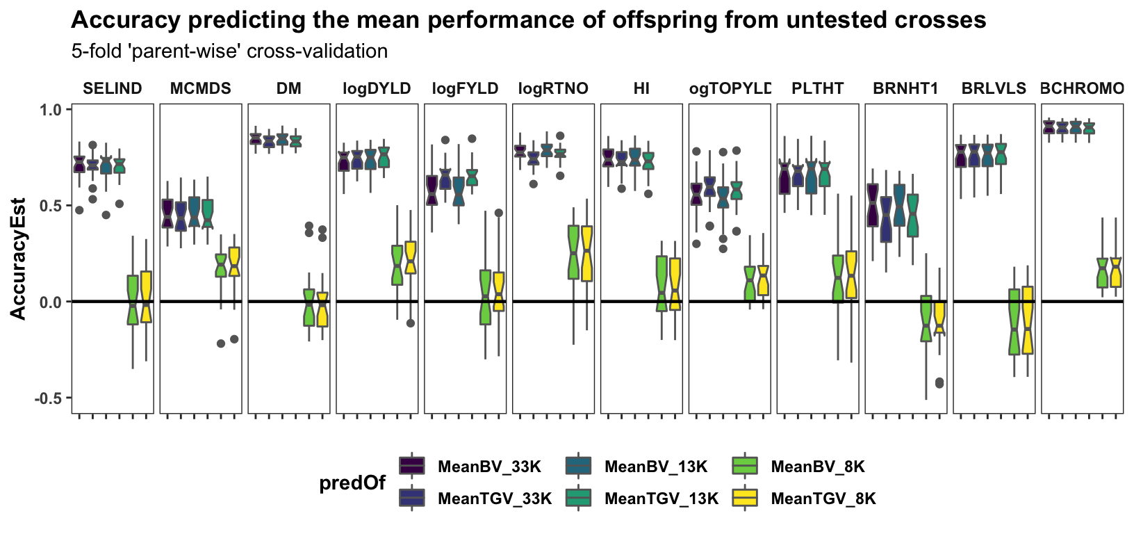

Past versions of unnamed-chunk-25-1.png

Version	Author	Date
e029efc	wolfemd	2021-08-12
f0a71e4	wolfemd	2021-08-11
cc1eb4b	wolfemd	2021-07-14

Cross-variance pred. accuracy

recalculated_accuracy %>% 
  filter(predOf=="Var",
         Trait1==Trait2) %>% 
  mutate(Trait1=factor(Trait1,levels=c("SELIND",blups$Trait)),
         predOf=factor(paste0("Var",VarComp,"_",Filter),
                       levels=c("VarBV_33K","VarTGV_33K","VarBV_13K","VarTGV_13K","VarBV_8K","VarTGV_8K"))) %>% 
  ggplot(.,aes(x=predOf,y=AccuracyEst,fill=predOf,color=Filter)) + 
  geom_boxplot(notch = TRUE,color='gray40') +
  scale_fill_manual(values = viridis::viridis(6)) + 
  scale_color_manual(values = viridis::viridis(6)) + 
  geom_hline(yintercept = 0, color='black', size=0.8) +
  facet_grid(.~Trait1) + 
  labs(title="Accuracy predicting variance in performance among offspring of untested crosses",
       subtitle="5-fold 'parent-wise' cross-validation") + 
  theme_bw() + 
  theme(axis.text.x = element_blank(),
        axis.title.x = element_blank(),
        strip.background = element_blank(),
        panel.grid.major = element_blank(),
        panel.grid.minor = element_blank(),
        legend.position='bottom',
        axis.text.y = element_text(face='bold'),
        axis.title.y = element_text(face='bold'),
        strip.text.x = element_text(face='bold'),
        plot.title = element_text(face='bold'),
        legend.title = element_text(face='bold'),
        legend.text = element_text(face='bold'),
        panel.spacing = unit(0.2, "lines"))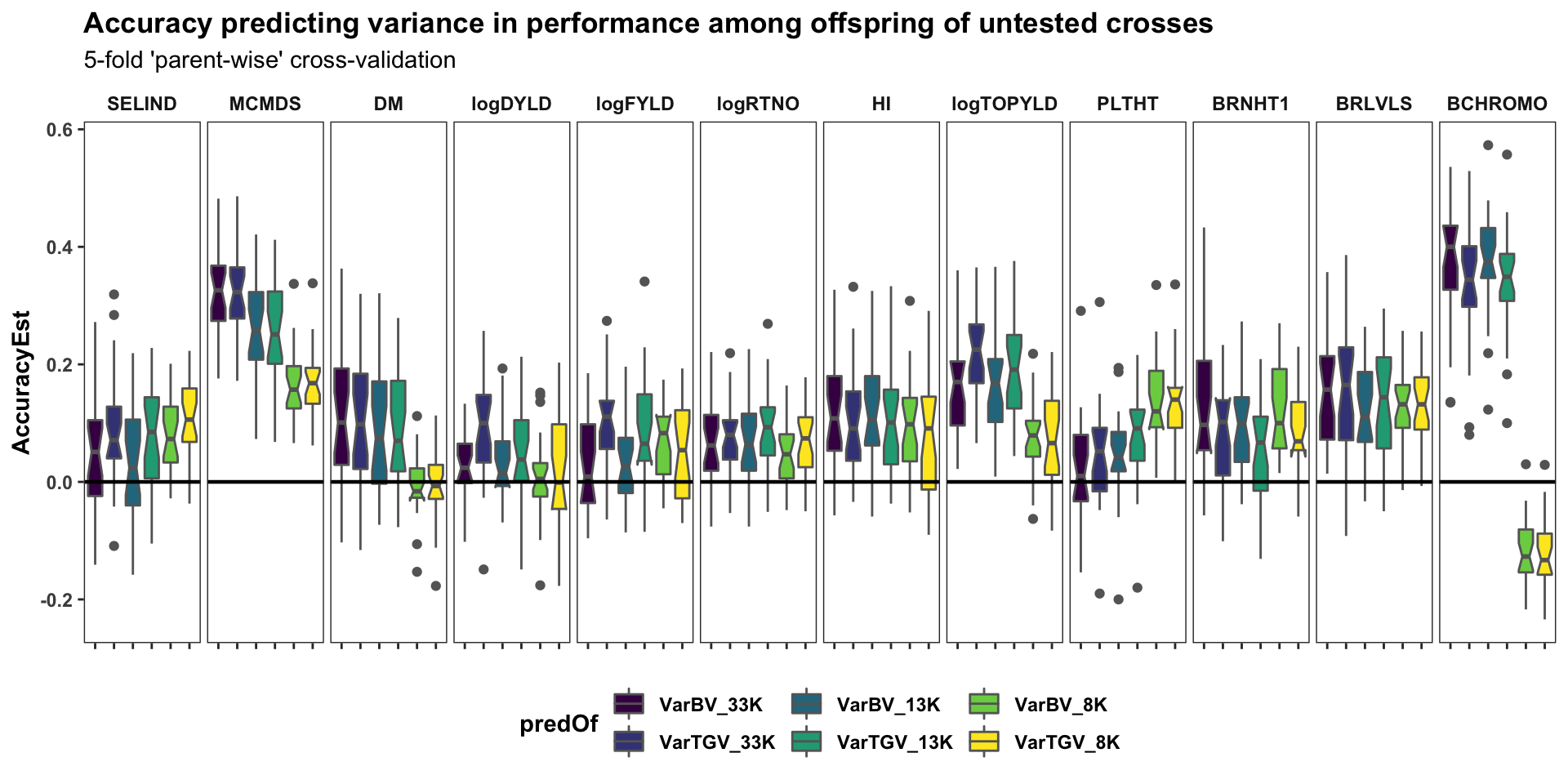

Past versions of unnamed-chunk-26-1.png

Version	Author	Date
e029efc	wolfemd	2021-08-12
f0a71e4	wolfemd	2021-08-11
cc1eb4b	wolfemd	2021-07-14

Cross-co-variance pred. accuracy

recalculated_accuracy %>% 
  filter(predOf=="Var",
         Trait1!=Trait2) %>% 
  mutate(Trait1=factor(Trait1,levels=c("SELIND",blups$Trait)),
         Trait2=factor(Trait2,levels=c("SELIND",blups$Trait)),
         predOf=factor(paste0("Var",VarComp,"_",Filter),
                       levels=c("VarBV_33K","VarTGV_33K","VarBV_13K","VarTGV_13K","VarBV_8K","VarTGV_8K"))) %>% 
  ggplot(.,aes(x=predOf,y=AccuracyEst,fill=predOf,color=Filter)) + 
  geom_boxplot(notch = TRUE) +
  scale_fill_manual(values = viridis::viridis(6)) + 
  scale_color_manual(values = viridis::viridis(6)) + 
  geom_hline(yintercept = 0, color='gray40', size=0.6) +
  facet_wrap(~Trait1+Trait2,nrow=5) + 
  labs(title="Accuracy predicting covariance in trait-trait performance within previously untested families",
       subtitle="5-fold 'parent-wise' cross-validation") + 
theme_bw() + 
  theme(axis.text.x = element_blank(),
        axis.title.x = element_blank(),
        strip.background = element_blank(),
        panel.grid.major = element_blank(),
        panel.grid.minor = element_blank(),
        legend.position='bottom',
        axis.text.y = element_text(face='bold'),
        axis.title.y = element_text(face='bold'),
        strip.text.x = element_text(face='bold'),
        plot.title = element_text(face='bold'),
        legend.title = element_text(face='bold'),
        legend.text = element_text(face='bold'),
        panel.spacing = unit(0.2, "lines"))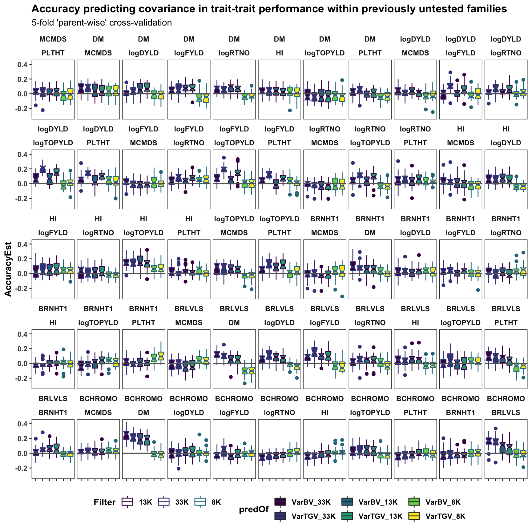

Past versions of unnamed-chunk-27-1.png

Version	Author	Date
e029efc	wolfemd	2021-08-12

rm(list=ls())

Genomic Predictions

After evaluating prediction accuracy, the genomic prediction step implements full-training dataset predictions and outputs tidy tables of selection criteria, including rankings on the selection index.

Selection of a subset of parents among which to predict matings: Went to cassavabase wizard, made a list of all IITA accessions in field trials dated 2020 and 2021 at 4 locations (IBA, IKN, MOK, UBJ), as these can likely source for crossing nurseries. I then used the SELIND GEBV and/or GETGV to rank all clones in the dataset (not just those “likely in field”). Goal is to pick more parents than we really want to cross, then predict the huge number of possible crosses, select the top crosses and then plan the corresponding parents into the crossing nursery. Conditional on the “likely in field list” I ended up with 200 parents-to-predict.

SNP sets: With the full_set (~31K SNP) predict cross-means only. With the medium_set (~13K SNP) predict cross-means and variances. We find high cor(full_set,medium_set) for the cross-means, and therefore will select the crosses based on means predicted with all SNP and variances predicted with medium set.

• Download CSV of genomic predictions here: Standard genomic predictions of the individual GEBV and GETGV for all selection candidates. Use for parent and/or clone selection.
• Download CSV of genomic mate predictions here: Genomic predictions of cross means, variance and usefulness on the selection index and for component traits. Cross mean predictions from full_set and variance predictions from medium_set.

Genetic trends (and gain estimates)

Plot genetic trends using selection index GEBV and GETGV of the individuals in the population.

# GBLUPs
### Two models AD and DirDom
gpreds_full<-readRDS(file = here::here("output","genomicPredictions_full_set_2021Aug09.rds"))
si_getgvs<-gpreds_full$gblups[[1]] %>% 
  filter(predOf=="GETGV") %>% 
  select(GID,SELIND)

## IITA Germplasm Ages
ggcycletime<-readxl::read_xls(here::here("data","PedigreeGeneticGainCycleTime_aafolabi_01122020.xls")) %>% 
  mutate(Year_Accession=as.numeric(Year_Accession))

# Need germplasmName field from raw trial data to match GEBV and cycle time
rawdata<-readRDS(here::here("output","IITA_ExptDesignsDetected_2021Aug08.rds"))
for_trend_plot<-si_getgvs %>% 
  left_join(rawdata %>% 
              distinct(germplasmName,GID)) %>% 
  group_by(GID) %>% 
  slice(1) %>% 
  ungroup()
# table(ggcycletime$Accession %in% si_getgvs$germplasmName)
# FALSE  TRUE 
#   193   614 

for_trend_plot %<>% 
  left_join(.,ggcycletime %>% 
              rename(germplasmName=Accession) %>% 
              mutate(Year_Accession=as.numeric(Year_Accession))) %>% 
  mutate(Year_Accession=case_when(grepl("2013_|TMS13",germplasmName)~2013,
                                  grepl("TMS14",germplasmName)~2014,
                                  grepl("TMS15",germplasmName)~2015,
                                  grepl("TMS16",germplasmName)~2016,
                                  grepl("TMS17",germplasmName)~2017,
                                  grepl("TMS18",germplasmName)~2018,
                                  grepl("TMS19",germplasmName)~2019,
                                  grepl("TMS20",germplasmName)~2020,
                                  !grepl("2013_|TMS13|TMS14|TMS15|TMS16|TMS17|TMS18|TMS19|TMS20",germplasmName)~Year_Accession))

# Declare the "eras" as PreGS\<2012 and GS\>=2013.
for_trend_plot %<>% 
  filter(Year_Accession>2012 | Year_Accession<2005)
for_trend_plot %<>% 
  mutate(GeneticGroup=ifelse(Year_Accession>=2013,"GS","PreGS"))

plottheme<-theme_bw() + 
  theme(axis.text.x = element_blank(),
        axis.title.x = element_blank(),
        strip.background = element_blank(),
        panel.grid.major = element_blank(),
        panel.grid.minor = element_blank(),
        legend.position='bottom',
        axis.text.y = element_text(face='bold'),
        axis.title.y = element_text(face='bold'),
        strip.text.x = element_text(face='bold'),
        plot.title = element_text(face='bold'),
        legend.title = element_text(face='bold'),
        legend.text = element_text(face='bold'),
        panel.spacing = unit(0.2, "lines")) 

First, for the IITA population, I use historical data on age of clones to perform a regression of GETGV on year-cloned compared the post 2012 (GS) to pre-GS era. The plot below shows the GETGV (y-axis) versus the year each accession was cloned.

for_trend_plot %>% 
  select(GeneticGroup,GID,Year_Accession,SELIND) %>% 
  ggplot(.,aes(x=Year_Accession,y=SELIND,color=GeneticGroup)) + 
  geom_point(size=1.25) + 
  geom_smooth(method=lm, se=TRUE, size=1.5) + 
  plottheme + theme(panel.grid.major = element_line()) + 
  scale_color_viridis_d() + 
  labs(title = "Selection Index GETGV vs. Accession Age by 'era' [GS vs. PreGS]",
       subtitle = "SI GETGV from modelType='DirDom'")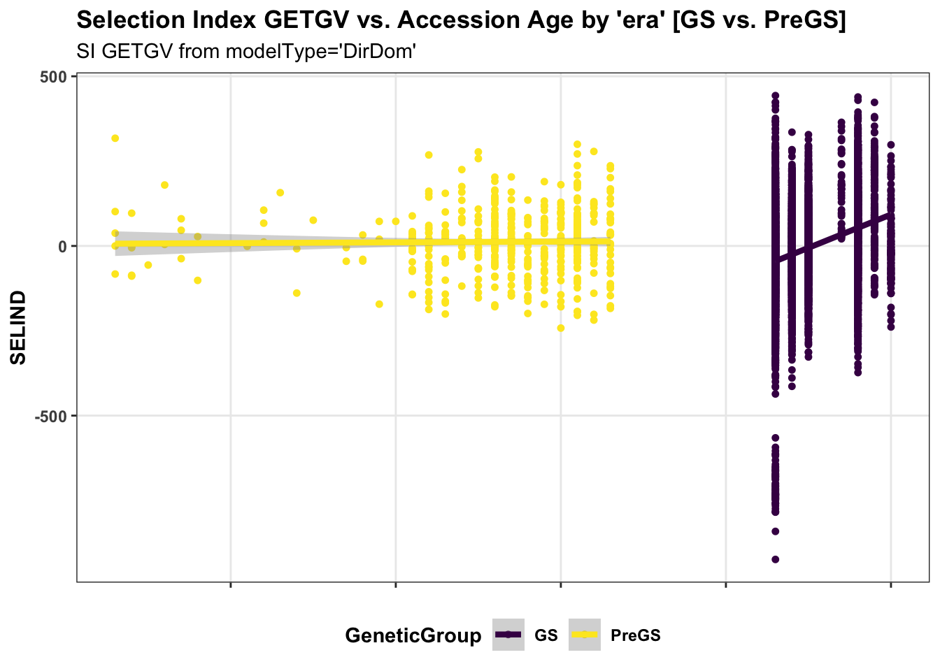 

Past versions of unnamed-chunk-30-1.png

Version	Author	Date
e029efc	wolfemd	2021-08-12
f0a71e4	wolfemd	2021-08-11
cc1eb4b	wolfemd	2021-07-14

Next, some fancy boxplot / half-violin plots to compare the distribution of GETGV across the cycles.

si_getgvs %>% 
  mutate(Cohort=NA,
         Cohort=ifelse(grepl("TMS20",GID,ignore.case = T),"TMS20",
                       ifelse(grepl("TMS19",GID,ignore.case = T),"TMS19",
                              ifelse(grepl("TMS18",GID,ignore.case = T),"TMS18",
                                     ifelse(grepl("TMS17",GID,ignore.case = T),"TMS17",
                                            ifelse(grepl("TMS16",GID,ignore.case = T),"TMS16",
                                                   ifelse(grepl("TMS15",GID,ignore.case = T),"TMS15",
                                                          ifelse(grepl("TMS14",GID,ignore.case = T),"TMS14",
                                                                 ifelse(grepl("TMS13|2013_",GID,ignore.case = T),"TMS13","PreGS")))))))),
         
         Cohort=factor(Cohort,levels = c("PreGS","TMS13","TMS14","TMS15","TMS16","TMS17","TMS18","TMS19","TMS20"))) %>% 
  ggplot(.,aes(x=Cohort,y=SELIND,fill=Cohort)) + 
  ggdist::stat_halfeye(adjust=0.5,.width = 0,fill='gray',width=0.75) +  
  geom_boxplot(width=0.12,notch = TRUE) +
  ggdist::stat_dots(side = "left",justification = 1.1,
                    binwidth = 0.03,dotsize=0.6) + 
  plottheme + 
  scale_fill_viridis_d()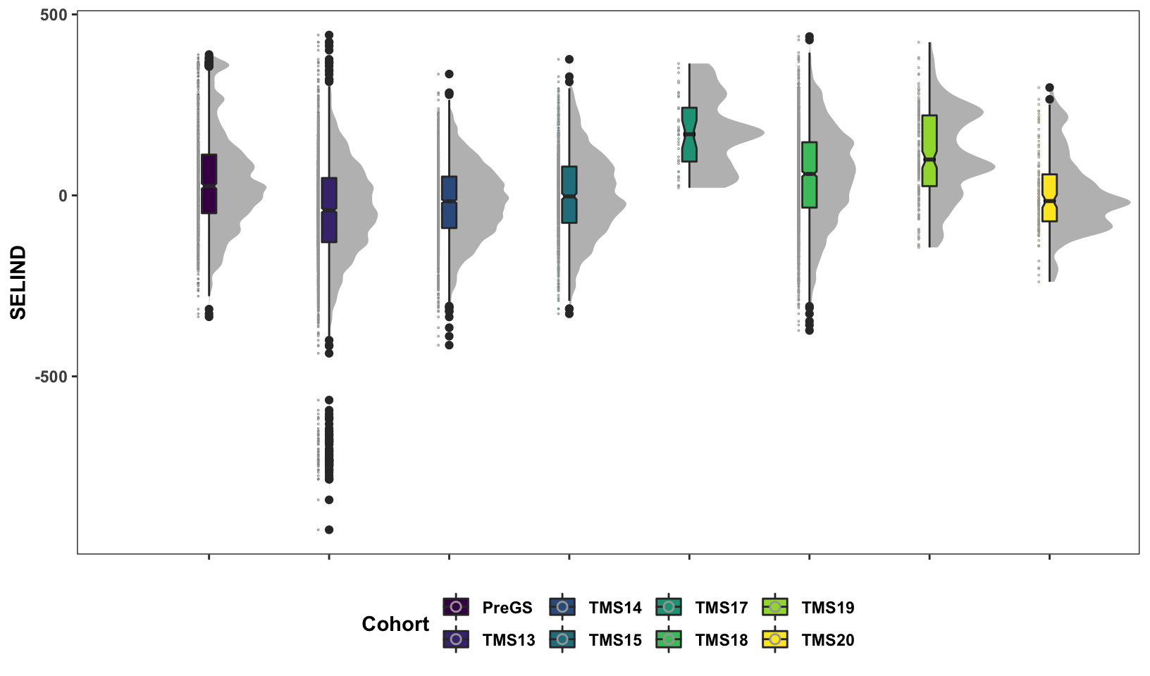

Past versions of unnamed-chunk-31-1.png

Version	Author	Date
e029efc	wolfemd	2021-08-12
f0a71e4	wolfemd	2021-08-11

Lastly, for continuity sake, barplots of the mean +/- std. error of GEBV across the cycles.

si_gebvs<-gpreds_full$gblups[[1]] %>% 
  filter(predOf=="GEBV") %>% 
  select(GID,SELIND) %>% 
  mutate(Cohort=NA,
         Cohort=ifelse(grepl("TMS20",GID,ignore.case = T),"TMS20",
                       ifelse(grepl("TMS19",GID,ignore.case = T),"TMS19",
                              ifelse(grepl("TMS18",GID,ignore.case = T),"TMS18",
                                     ifelse(grepl("TMS17",GID,ignore.case = T),"TMS17",
                                            ifelse(grepl("TMS16",GID,ignore.case = T),"TMS16",
                                                   ifelse(grepl("TMS15",GID,ignore.case = T),"TMS15",
                                                          ifelse(grepl("TMS14",GID,ignore.case = T),"TMS14",
                                                                 ifelse(grepl("TMS13|2013_",GID,ignore.case = T),"TMS13","PreGS")))))))),
         
         Cohort=factor(Cohort,levels = c("PreGS","TMS13","TMS14","TMS15","TMS16","TMS17","TMS18","TMS19","TMS20")))
si_gebvs %>% 
  group_by(Cohort) %>% 
  summarize(meanGEBV=mean(SELIND),
            stdErr=sd(SELIND)/sqrt(n()),
            upperSE=meanGEBV+stdErr,
            lowerSE=meanGEBV-stdErr) %>% 
  ggplot(.,aes(x=Cohort,y=meanGEBV,fill=Cohort)) + 
  geom_bar(stat = 'identity', color='gray60', size=1.25) + 
  geom_linerange(aes(ymax=upperSE,
                     ymin=lowerSE), color='gray60', size=1.25) + 
  #facet_wrap(~Trait,scales='free_y', ncol=1) + 
  theme_bw() +
  geom_hline(yintercept = 0, size=1.15, color='black') + 
  plottheme + 
  scale_fill_viridis_d() + 
  labs(x=NULL,y="Mean GEBVs",
       title="Mean +/- Std. Error Selection Index GEBV by Annual Cohort")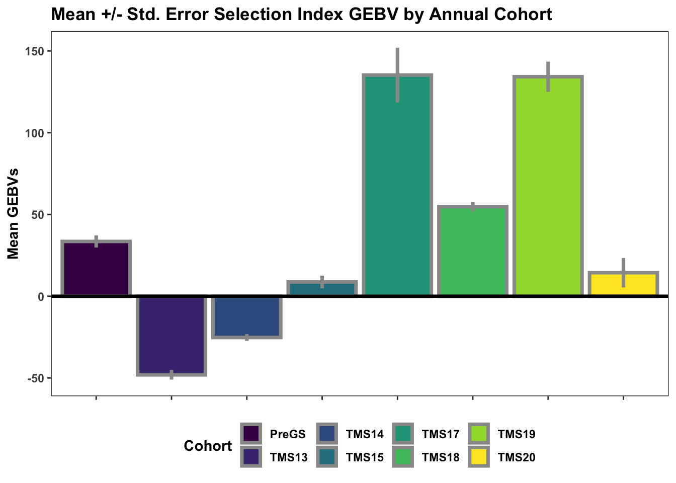

Past versions of unnamed-chunk-32-1.png

Version	Author	Date
e029efc	wolfemd	2021-08-12

Parents selected for cross predictions

I predicted 20100 crosses of 200 elite candidate parents.

Below is a plot showing the distribution of GETGV for the entire population contrasted to the selected set of parents. Fill color indicates Cohort.

library(tidyverse); library(magrittr); library(ggdist)
parentsToPredictCrosses<-readRDS(file = here::here("output",
                                                   "parentsToPredictCrosses_2021Aug10.rds"))
for_selected_plot<-si_getgvs %>% 
  mutate(Cohort=NA,
         Cohort=ifelse(grepl("TMS20",GID,ignore.case = T),"TMS20",
                       ifelse(grepl("TMS19",GID,ignore.case = T),"TMS19",
                              ifelse(grepl("TMS18",GID,ignore.case = T),"TMS18",
                                     ifelse(grepl("TMS17",GID,ignore.case = T),"TMS17",
                                            ifelse(grepl("TMS16",GID,ignore.case = T),"TMS16",
                                                   ifelse(grepl("TMS15",GID,ignore.case = T),"TMS15",
                                                          ifelse(grepl("TMS14",GID,ignore.case = T),"TMS14",
                                                                 ifelse(grepl("TMS13|2013_",GID,ignore.case = T),"TMS13","PreGS")))))))),
         
         Cohort=factor(Cohort,levels = c("PreGS","TMS13","TMS14","TMS15","TMS16","TMS17","TMS18","TMS19","TMS20")))
for_selected_plot %>% 
  mutate(Cycle="AllGermplasm") %>% 
  bind_rows(for_selected_plot %>% 
              filter(GID %in% parentsToPredictCrosses) %>% 
              mutate(Cycle="SelectedParents")) %>% 
  mutate(Cycle=factor(Cycle,levels = c("AllGermplasm","SelectedParents"))) %>% 
  ggplot(.,aes(x=Cycle,y=SELIND,fill=Cycle)) + 
  ggdist::stat_halfeye(adjust=0.5,.width = 0,fill='gray',width=0.75) +  
  geom_boxplot(width=0.09,notch = TRUE) +
  ggdist::stat_dots(aes(color=Cohort),side = "left",justification = 1.1,dotsize=.8) + 
  scale_fill_viridis_d() + scale_color_viridis_d() + 
  plottheme + 
  labs(title="Distribution of selection index GETGV in parents selected for mate predictions",
       subtitle="compared to the overall population")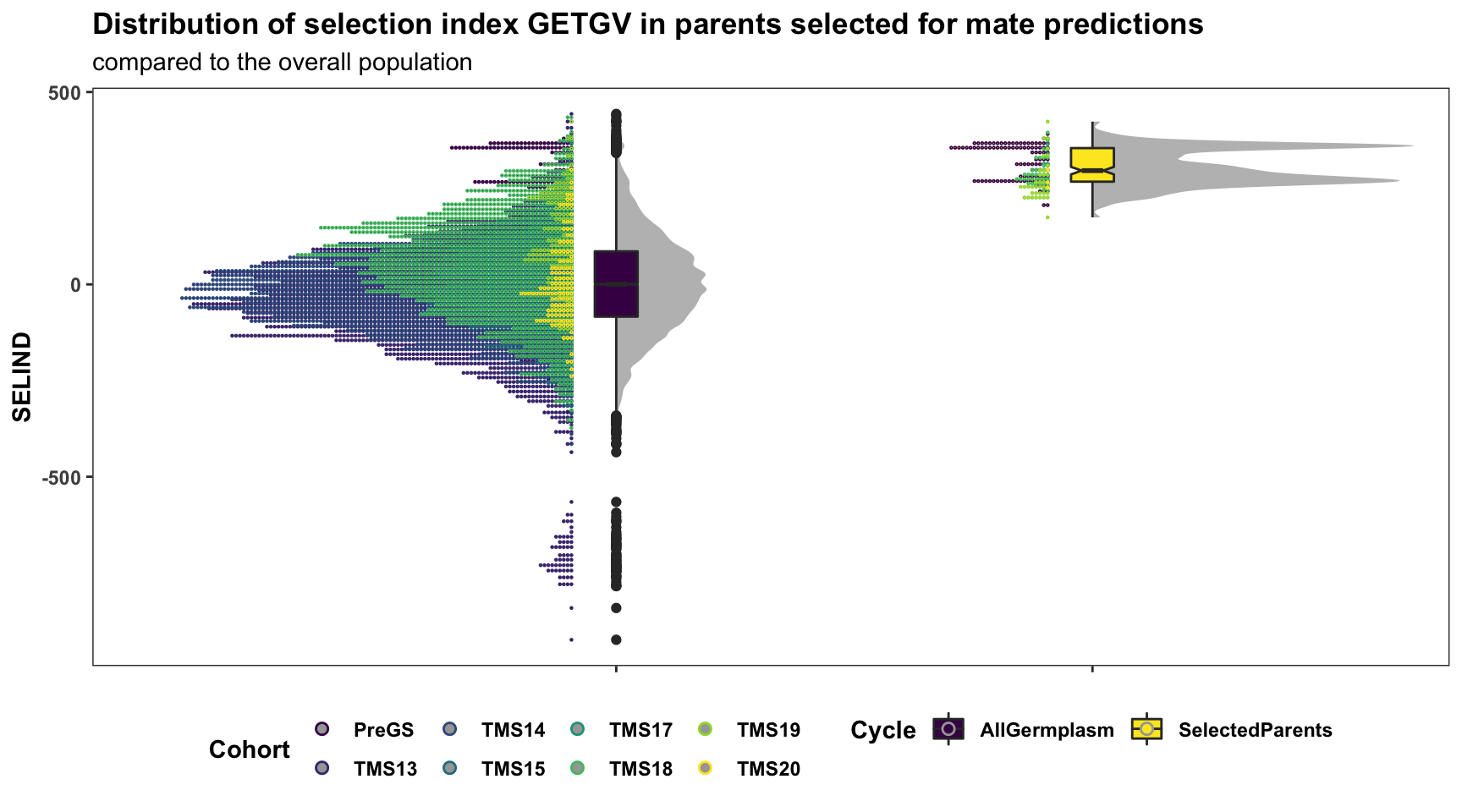

Past versions of unnamed-chunk-33-1.png

Version	Author	Date
e029efc	wolfemd	2021-08-12

for_selected_plot %>% 
  filter(GID %in% parentsToPredictCrosses) %>% 
  count(Cohort, name = "NparentsToPredCrosses")

# A tibble: 7 × 2
  Cohort NparentsToPredCrosses
  <fct>                  <int>
1 PreGS                    109
2 TMS13                      1
3 TMS14                      1
4 TMS17                      9
5 TMS18                     39
6 TMS19                     38
7 TMS20                      3

Surprisingly, a significant amount of parents from the “PreGS” (i.e. GeneticGain pop. clones is recommended). Not sure that is what we will actually want to do in practice, but it makes sense when viewed in light of the rankings plotted above: they still have elite GEBV/GETGV.

Genomic mate selection

Update: September 18th, 2021: completed predicting 258840 pairwise crosses among 719 in-field parents.

library(tidyverse); library(magrittr); library(ggdist)
crossPreds<-read.csv(here::here("output","genomicMatePredictions_2021Sep18.csv"), stringsAsFactors = F, header = T)

forplot<-crossPreds %>% 
  filter(Trait=="SELIND") %>% 
  select(sireID,damID,CrossGroup,predOf,predMean,predSD,predUsefulness)

cross_group_order<-crossPreds %>% 
  filter(Trait=="SELIND") %>% 
  distinct(sireGroup,damGroup) %>% 
  mutate(sireGroup=factor(sireGroup,levels=c("PreGS","TMS13","TMS14","TMS15","TMS16","TMS17","TMS18","TMS19","TMS20")),
         damGroup=factor(damGroup,levels=c("PreGS","TMS13","TMS14","TMS15","TMS16","TMS17","TMS18","TMS19","TMS20"))) %>% 
  arrange(desc(sireGroup),desc(damGroup)) %>% 
  mutate(CrossGroup=paste0(sireGroup,"x",damGroup)) %$% 
  CrossGroup

forplot %<>% 
  mutate(CrossGroup=factor(CrossGroup,levels=c(cross_group_order)))

The standard budget for genotyping has been 2500 new clones per year.

Suppose we choose to create 50 families of 50 siblings each, from the 20100 predicted crosses.

The input file has a pre-computed predUsefulness variable. I used stdSelInt=2.062 when making the predictions with the predictCrosses() function, which corresponds to selecting the top 5% (or top 5 offspring) from each family.

Crosses may be of interest for their predicted \(UC_{parent}\) (predOf=="BV") and/or \(UC_{variety}\) (predOf=="TGV").

Each crossing nursery needs to produce both new exceptional parents and elite candidate cultivars. These will not necessarily be the same individuals or come from the same crosses.

forplot %>%
  select(-predMean,-predSD) %>%
  spread(predOf,predUsefulness) %$%
  cor(BV,TGV)

[1] 0.9687978

# [1] 0.9687978
# The correlation between predUC BV and TGV is high.

forplot %>%
  group_by(predOf) %>%
  slice_max(order_by = predUsefulness, n = 50) %>% ungroup() %>%
  distinct(sireID,damID) %>% nrow() # 71

[1] 71

The correlation between predUC BV and TGV is higher among this total group of cross predictions with moderate overlap between crosses seleccted for both \(UC_{parent}\) (predOf=="BV") and/or \(UC_{variety}\) (predOf=="TGV").

forplot %>% 
  filter(predOf=="TGV") %>% 
  sample_n(2000) %>% 
#  slice_max(order_by = predUsefulness, n = 1000) %>% 
  arrange(desc(predUsefulness)) %>% 
  mutate(Rank=1:nrow(.)) %>% 
  ggplot(aes(x = Rank, dist = "norm", 
             arg1 = predMean, arg2 = predSD, 
             fill=CrossGroup, color=CrossGroup),
         alpha=0.5) +
  stat_dist_pointinterval() +
  #stat_dist_gradientinterval(n=50) +
  scale_fill_viridis_d() + scale_color_viridis_d() + 
  plottheme + theme(axis.title.x = element_text(face='bold')) + 
  labs(x = "Cross Rank UC_variety",
       y = "Selection Index GETGV",
       title = "Predicted distribution (mean and variability) of a sample of 2000 of 258840 predicted crosses",
       subtitle = "Gives an idea of the range")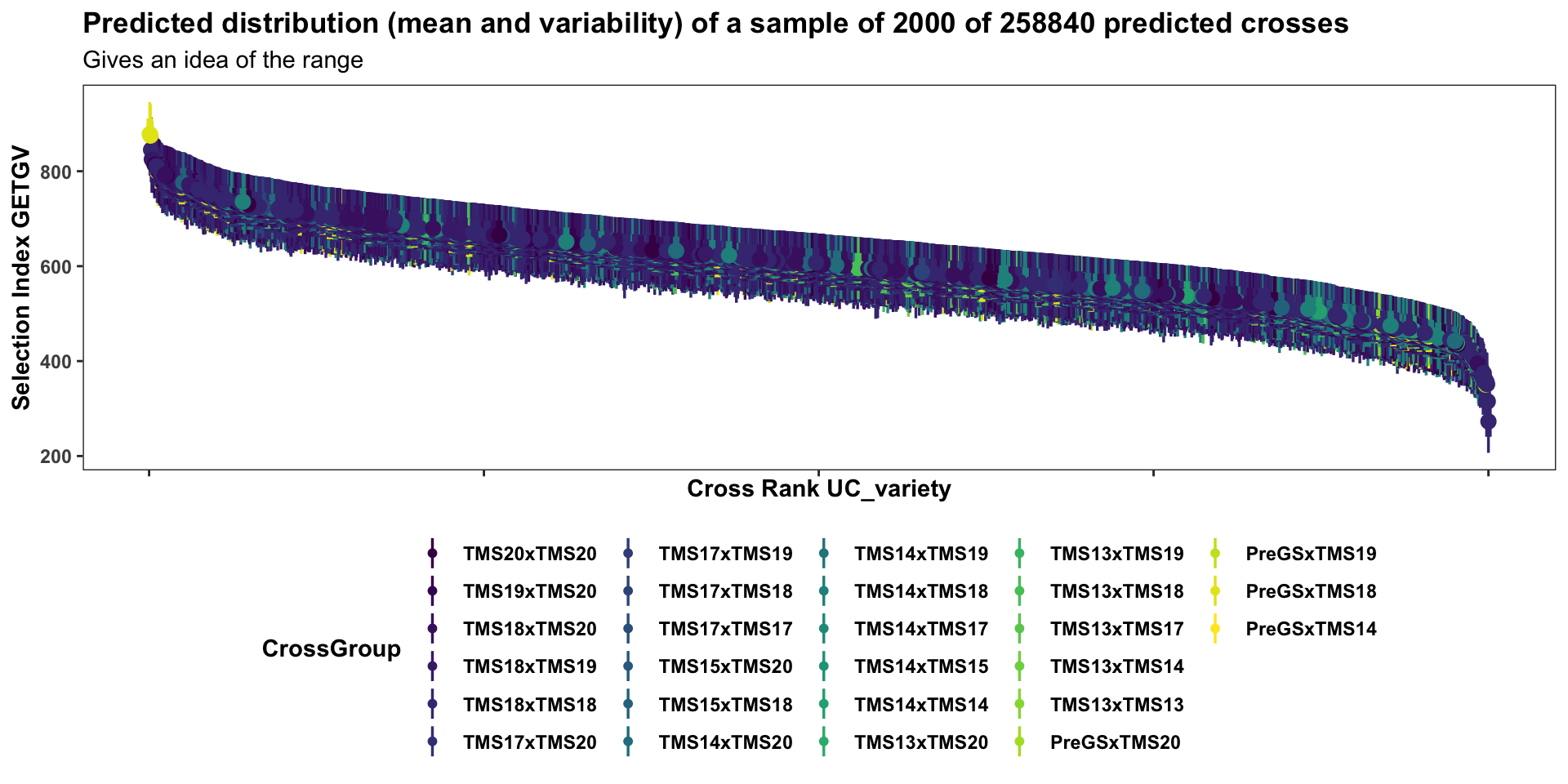

Past versions of unnamed-chunk-37-1.png

Version	Author	Date
e029efc	wolfemd	2021-08-12

forplot %>% 
  filter(predOf=="BV") %>% 
  sample_n(2000) %>% 
  #slice_max(order_by = predUsefulness, n = 100) %>% 
  arrange(desc(predUsefulness)) %>% 
  mutate(Rank=1:nrow(.)) %>% 
  ggplot(aes(x = Rank, dist = "norm", 
             arg1 = predMean, arg2 = predSD, 
             fill=CrossGroup, color=CrossGroup),
         alpha=0.5) +
  stat_dist_pointinterval() +
  #stat_dist_gradientinterval(n=50) +
  scale_fill_viridis_d() + scale_color_viridis_d() + 
  plottheme + theme(axis.title.x = element_text(face='bold')) + 
  labs(x = "Cross Rank UC_parent",
       y = "Selection Index GEBV",
       title = "Predicted distribution (mean and variability) of a sample of 2000 of 258840 predicted crosses",
       subtitle = "Gives an idea of the range")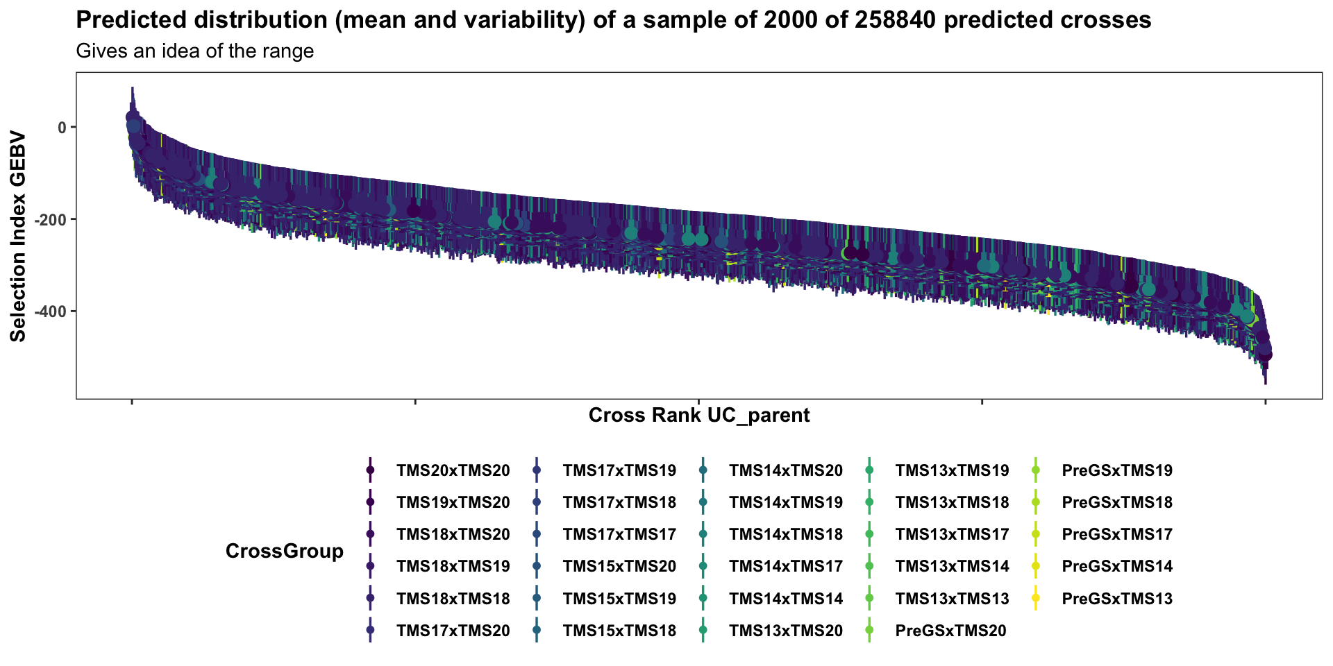

Past versions of unnamed-chunk-38-1.png

Version	Author	Date
e029efc	wolfemd	2021-08-12

This first two plots of the mate predictions display the entire set of predicted crosses, ranked by their selection index \(UC^{SI}_{variety}\) and \(UC^{SI}_{parent}\) respectively. This will be more clear in the subsequent plots with fewer families: the x-axis is simply the descending rank of predicted \(UC^{SI}\) for each cross. The y-axis shows the predicted mean (dot) and distribution quantiles (linerange) based on the predicted mean and standard deviation of each cross. Crosses are color coded according to the “genetic group” of the parents.

forplot %>% 
  group_by(predOf) %>% 
  slice_max(order_by = predUsefulness, n = 100) %>% 
  arrange(predOf,desc(predUsefulness)) %>% 
  group_by(predOf) %>% 
  mutate(Rank=1:n()) %>% 
    ggplot(aes(x = Rank, dist = "norm", 
               arg1 = predMean, arg2 = predSD, 
               fill=CrossGroup, color=CrossGroup),
           alpha=1) +
    stat_dist_gradientinterval(n=100) +
    scale_fill_viridis_d() + scale_color_viridis_d() + 
  plottheme + theme(axis.text.x = element_text(face='bold'),
                    axis.title.x = element_text(face = 'bold')) + 
  facet_wrap(~predOf,nrow=1, scales='free') + 
  labs(x = "Selection Index Ranking",
       y = "Selection Index GBLUP",
       title = "Predicted distribution of the top 100 crosses")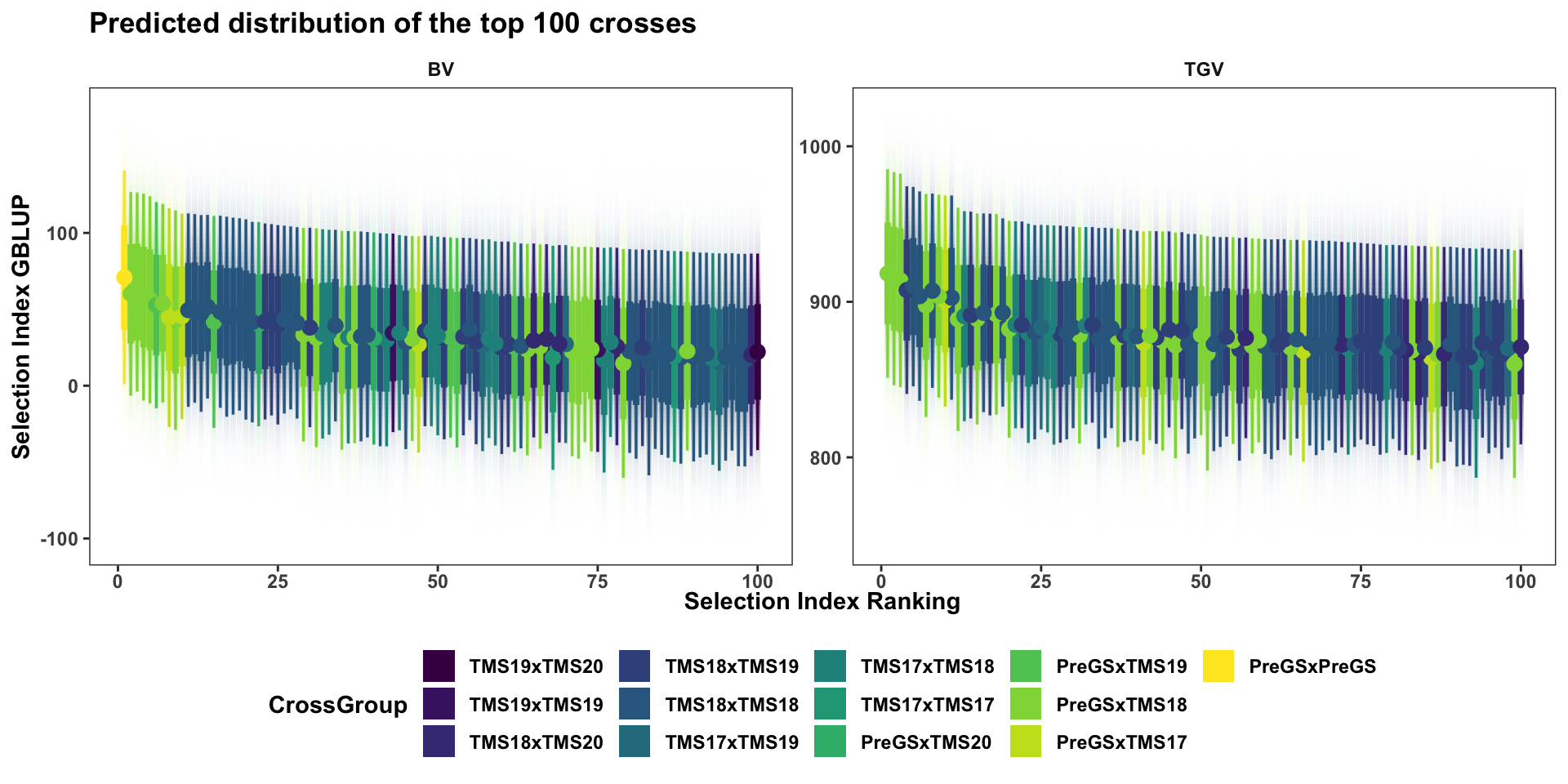

Past versions of unnamed-chunk-39-1.png

Version	Author	Date
e029efc	wolfemd	2021-08-12

This next plot shows only the top 100 crosses, ranked separately based on the \(UC^{SI}_{parent}\) and \(UC^{SI}_{variety}\).

forplot %>% 
  group_by(predOf) %>% 
  slice_max(order_by = predUsefulness, n = 5) %>% rmarkdown::paged_table()

The best 5 crosses to make based on \(UC^{SI}_{parent}\) and \(UC^{SI}_{variety}\):

forplot %>% 
  group_by(predOf) %>% 
  slice_max(order_by = predUsefulness, n = 50) %>% 
  arrange(predOf,desc(predUsefulness)) %>% 
  mutate(Rank=1:n()) %>% 
  ggplot(aes(x = Rank, dist = "norm", 
             arg1 = predMean, arg2 = predSD, 
             fill = CrossGroup,
             label = CrossGroup)) +
  stat_dist_gradientinterval(n=100,side='top',position = "dodgejust",
                         aes(fill = stat(y < (arg1+arg2*qnorm(0.95))))) +
  stat_dist_dotsinterval(n=50,side='both',position = "dodgejust",
                         aes(fill = stat(y < (arg1+arg2*qnorm(0.95))))) +
  scale_fill_viridis_d() + scale_color_viridis_d() + 
  plottheme + theme(axis.text.x = element_text(face='bold'),
                    axis.title.x = element_text(face = 'bold'),
                    legend.position = 'none') + 
  facet_wrap(~predOf,nrow=2, scales='free') + 
  labs(x = expression(bold("Rank on SELIND")),
       y = "Selection Index GBLUP",
       title = "Predicted distribution of the top 50 crosses")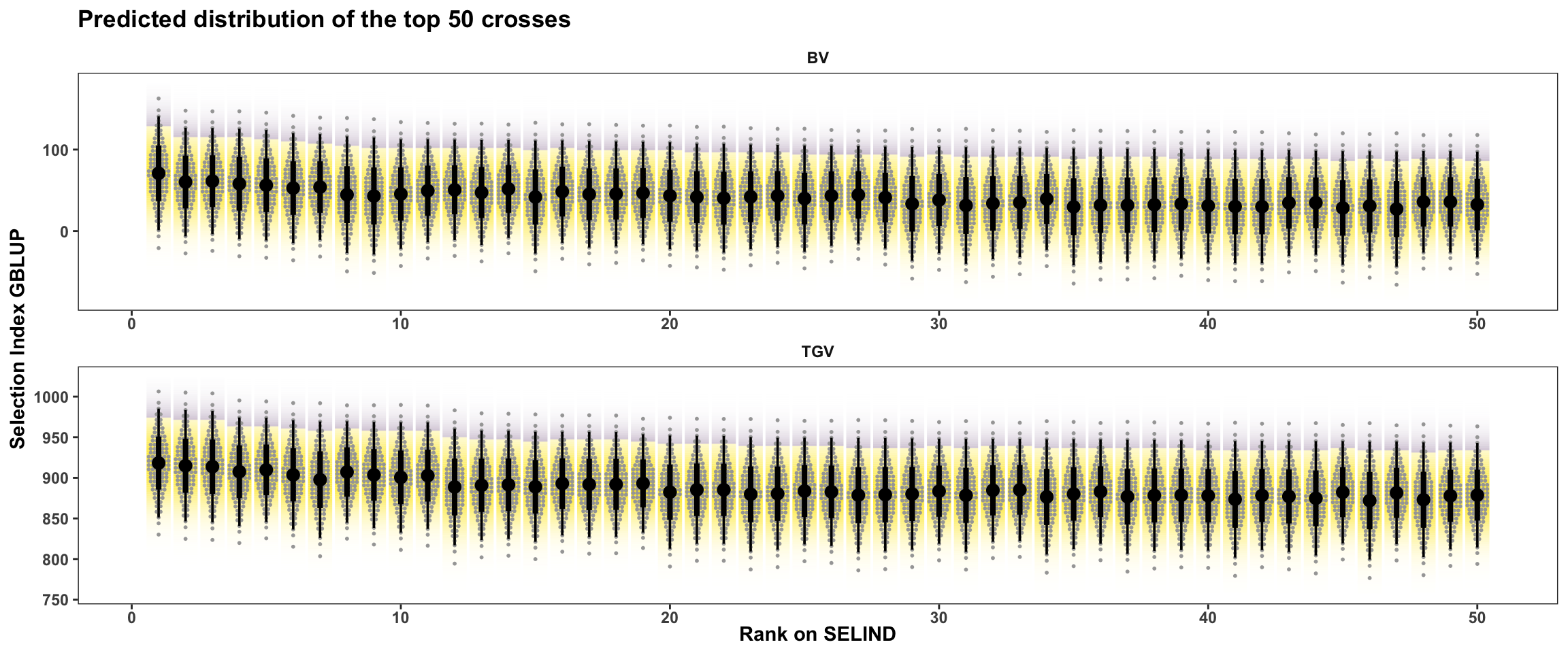

Past versions of unnamed-chunk-41-1.png

Version	Author	Date
e029efc	wolfemd	2021-08-12

In this plot, the area under the top 5% of each crosses predicted distribution is filled in purple The mean of individuals from under the highlighted area is the \(UC_{parent}\) or \(UC_{variety}\). There are also 50 dots for each cross illustrating the hypothetical outcome of creating 50 progeny.

forplot %>% 
  group_by(predOf) %>% 
  slice_max(order_by = predUsefulness, n = 10) %>% 
  arrange(predOf,desc(predUsefulness)) %>% 
  mutate(Rank=1:n()) %>% 
  ggplot(aes(y = Rank, dist = "norm", 
             arg1 = predMean, arg2 = predSD, 
             label = paste0(sireID,"\n x ",damID)),
         alpha=0.5) +
  stat_dist_dotsinterval(n=50,side='top',position = "dodgejust",scale=0.85,
                         aes(fill = stat(x < (arg1+arg2*qnorm(0.95))))) +
  stat_dist_halfeye(position = "dodgejust",scale=1.25, alpha=0.5,
                    aes(fill = stat(x < (arg1+arg2*qnorm(0.95))))) +
  geom_label(aes(x=predMean),size=3) + 
  scale_fill_viridis_d() + scale_color_viridis_d() + 
  plottheme + theme(axis.text.x = element_text(face='bold'),
                    axis.title.x = element_text(face = 'bold'),
                    legend.position = 'none') + 
  facet_wrap(~predOf,scales='free', nrow=1) + 
  labs(y = expression(bold("Rank on SELIND")),
       x = "Selection Index GBLUP",
       title = "Predicted distribution of the top 10 crosses")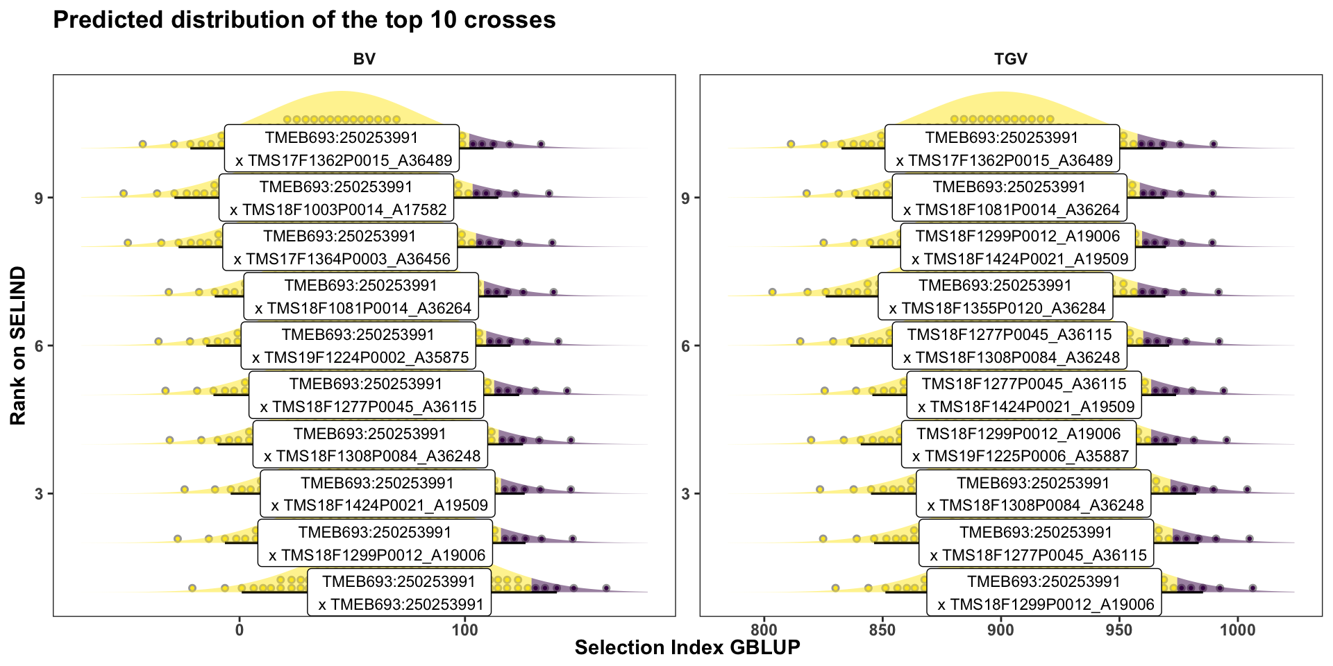

Past versions of unnamed-chunk-42-1.png

Version	Author	Date
e029efc	wolfemd	2021-08-12

Or for more clarity, just the top 10 crosses:

Selection Criteria and Recommendations

Table of Top 50 Crosses: 2 rows for each cross, one for predOf=="BV" one for predOf=="TGV".

• Download the CSV for the top 50 crosses and their selection index means, SDs and UC here or
• Download the complete CSV of ALL genomic mate predictions here: for all crosses and both SELIND and component trait predictions.

top50crosses<-forplot %>% 
  group_by(predOf) %>% 
  slice_max(order_by = predUsefulness, n = 50) %>% 
  ungroup()
top50crosses %>% 
  write.csv(.,file = here::here("output","top50crosses_2021Sep18.csv"), row.names = F)
top50crosses %>% 
  rmarkdown::paged_table()

For AM 2021

Plot SELIND prediction accuracy

library(tidyverse); library(magrittr); library(ggdist)
# PARENT-WISE CV RESULTS
accuracy_full<-readRDS(here::here("output","parentWiseCV_full_set_CrossPredAccuracy.rds"))
accuracy_medium<-readRDS(here::here("output","parentWiseCV_medium_set_CrossPredAccuracy.rds"))
accuracy_reduced<-readRDS(here::here("output","parentWiseCV_reduced_set_CrossPredAccuracy.rds"))
accuracy<-accuracy_medium$meanPredAccuracy %>%
  filter(Trait=="SELIND") %>%
  mutate(VarComp=gsub("Mean","",predOf),
         predOf="Mean",
         Filter="LDprunedR2pt8 \n (~13K)") %>%
  bind_rows(accuracy_medium$varPredAccuracy %>%
              filter(Trait1=="SELIND") %>%
              rename(Trait=Trait1) %>%
              select(-Trait2) %>%
              mutate(VarComp=gsub("Var","",predOf),
                     predOf="Var",
                     Filter="LDprunedR2pt8 \n (~13K)")) %>%
  bind_rows(accuracy_reduced$meanPredAccuracy %>%
  filter(Trait=="SELIND") %>%
  mutate(VarComp=gsub("Mean","",predOf),
         predOf="Mean",
         Filter="LDprunedR2pt6 \n (~8K)") %>%
  bind_rows(accuracy_reduced$varPredAccuracy %>%
              filter(Trait1=="SELIND") %>%
              rename(Trait=Trait1) %>%
              select(-Trait2) %>%
              mutate(VarComp=gsub("Var","",predOf),
                     predOf="Var",
                     Filter="LDprunedR2pt6 \n (~8K)"))) %>%
    bind_rows(accuracy_full$meanPredAccuracy %>%
  filter(Trait=="SELIND") %>%
  mutate(VarComp=gsub("Mean","",predOf),
         predOf="Mean",
         Filter="FullSet \n (~33K)") %>%
  bind_rows(accuracy_full$varPredAccuracy %>%
              filter(Trait1=="SELIND") %>%
              rename(Trait=Trait1) %>%
              select(-Trait2) %>%
              mutate(VarComp=gsub("Var","",predOf),
                     predOf="Var",
                     Filter="FullSet \n (~33K)")))

recalculated_accuracy<-accuracy %>% 
  select(-AccuracyEst) %>% 
  unnest(predVSobs) %>% 
  select(-obsVar,-obsMean,-obsVar) %>% 
  mutate(predValue=ifelse(predOf=="Mean",predMean,predVar)) %>% 
  select(-predVar,-predMean) %>% 
  left_join(accuracy %>% 
              select(-AccuracyEst) %>% 
              filter(grepl("FullSet",Filter)) %>% 
              unnest(predVSobs) %>% 
              select(-predVar,-predMean) %>% 
              mutate(obsValue=ifelse(predOf=="Mean",obsMean,obsVar)) %>% 
              select(-obsMean,-obsVar,-Filter)) %>% 
  nest(predVSobs=c(sireID,damID,predValue,obsValue,famSize)) %>% 
  mutate(AccuracyEst=map_dbl(predVSobs,function(predVSobs){
    out<-psych::cor.wt(predVSobs[,c("predValue","obsValue")],
                       w = predVSobs$famSize) %$% r[1,2] %>%
      round(.,3)
    return(out) })) %>% 
  select(-predVSobs)   

recalculated_accuracy %<>%
  filter(grepl("FullSet",Filter)) %>% 
  mutate(predOf=paste0("Cross",predOf))
  mutate(predOf=factor(predOf,levels=c("CrossMean","CrossVar")),
         VarComp=factor(VarComp,levels=c("BV","TGV"))) %>% droplevels

colors<-viridis::viridis(4)[1:2]

recalculated_accuracy %>% 
  ggplot(.,aes(x=VarComp,y=AccuracyEst,fill=VarComp)) +
  ggdist::stat_halfeye(adjust=0.5,.width = 0,fill='gray',width=0.75) +  
  geom_boxplot(width=0.12,notch = TRUE) +
  ggdist::stat_dots(side = "left",justification = 1.1,dotsize=0.6)+
  theme_bw() + 
  scale_fill_manual(values = colors) + 
  geom_hline(data = recalculated_accuracy %>% distinct(predOf) %>% mutate(yint=c(NA,0)),
             aes(yintercept = yint), color='black', size=0.9) +
  theme(axis.text.x = element_blank(),
        axis.title.x = element_blank(),
        strip.background = element_blank(),
        panel.grid.major = element_blank(),
        panel.grid.minor = element_blank(),
        axis.title = element_text(face='bold',color = 'black', size=14),
        strip.text.y = element_text(face='bold',color='black',size=16),
        axis.text.y = element_text(face = 'bold',color='black',size=12),
        legend.text = element_text(face='bold',size=14),
        legend.title = element_text(face='bold',size=14),
        legend.position = 'bottom',
        plot.title = element_text(face='bold',size=16)) +
  facet_grid(predOf~.,scales = 'free') + 
  labs(title="Accuracy predicting performance on the Selection Index") 

Session information

sessionInfo()

R version 4.1.1 (2021-08-10)
Platform: x86_64-apple-darwin17.0 (64-bit)
Running under: macOS Big Sur 10.16

Matrix products: default
BLAS:   /Library/Frameworks/R.framework/Versions/4.1/Resources/lib/libRblas.0.dylib
LAPACK: /Library/Frameworks/R.framework/Versions/4.1/Resources/lib/libRlapack.dylib

locale:
[1] en_US.UTF-8/en_US.UTF-8/en_US.UTF-8/C/en_US.UTF-8/en_US.UTF-8

attached base packages:
[1] stats     graphics  grDevices utils     datasets  methods   base     

other attached packages:
 [1] ggdist_3.0.0    ragg_1.1.3      magrittr_2.0.1  forcats_0.5.1  
 [5] stringr_1.4.0   dplyr_1.0.7     purrr_0.3.4     readr_2.0.1    
 [9] tidyr_1.1.3     tibble_3.1.4    ggplot2_3.3.5   tidyverse_1.3.1
[13] workflowr_1.6.2

loaded via a namespace (and not attached):
 [1] nlme_3.1-153         fs_1.5.0             lubridate_1.7.10    
 [4] httr_1.4.2           rprojroot_2.0.2      tools_4.1.1         
 [7] backports_1.2.1      bslib_0.3.0          utf8_1.2.2          
[10] R6_2.5.1             mgcv_1.8-36          DBI_1.1.1           
[13] colorspace_2.0-2     withr_2.4.2          gridExtra_2.3       
[16] tidyselect_1.1.1     mnormt_2.0.2         compiler_4.1.1      
[19] git2r_0.28.0         textshaping_0.3.5    cli_3.0.1           
[22] rvest_1.0.1          xml2_1.3.2           labeling_0.4.2      
[25] sass_0.4.0           scales_1.1.1         psych_2.1.6         
[28] systemfonts_1.0.2    digest_0.6.27        rmarkdown_2.11      
[31] pkgconfig_2.0.3      htmltools_0.5.2      dbplyr_2.1.1        
[34] fastmap_1.1.0        highr_0.9            rlang_0.4.11        
[37] readxl_1.3.1         rstudioapi_0.13      jquerylib_0.1.4     
[40] farver_2.1.0         generics_0.1.0       jsonlite_1.7.2      
[43] distributional_0.2.2 Matrix_1.3-4         Rcpp_1.0.7          
[46] munsell_0.5.0        fansi_0.5.0          viridis_0.6.1       
[49] lifecycle_1.0.0      stringi_1.7.4        whisker_0.4         
[52] yaml_2.2.1           grid_4.1.1           parallel_4.1.1      
[55] promises_1.2.0.1     crayon_1.4.1         lattice_0.20-44     
[58] splines_4.1.1        haven_2.4.3          hms_1.1.0           
[61] tmvnsim_1.0-2        knitr_1.34           pillar_1.6.2        
[64] reprex_2.0.1         glue_1.4.2           evaluate_0.14       
[67] modelr_0.1.8         vctrs_0.3.8          tzdb_0.1.2          
[70] httpuv_1.6.3         cellranger_1.1.0     gtable_0.3.0        
[73] assertthat_0.2.1     xfun_0.26            broom_0.7.9         
[76] later_1.3.0          viridisLite_0.4.0    ellipsis_0.3.2      
[79] here_1.0.1