library(genomicMateSelectR)
#> Loading required package: tibble
#> Loading required package: dplyr
#>
#> Attaching package: 'dplyr'
#> The following objects are masked from 'package:stats':
#>
#>     filter, lag
#> The following objects are masked from 'package:base':
#>
#>     intersect, setdiff, setequal, union
#> Loading required package: tidyr
#> Loading required package: purrr
The following will be a demonstration of the core functions for predicting mate selection criteria available in genomicMateSelectR.
Simulated data
I generated simulated data, included in the package (accessible via data()), which should clarify the input format(s) required.
The example input data will be explained and used in the vignette below.
Simulation was conducted with the package AlphaSimR.
- Simulate 100 individuals, 2 chrom., 100 seg. sites, 50 SNP/chr.
- 2 traits, gen. corr. 0.5, \(h^2=0.5\), 10 QTL/chr. equal parts additive + dominance.
- 2 cycles of phenotypic selection, based on one of the two traits, top 5 individuals, 10 crosses x 10 progeny
- Generates 300 individuals across 3 generations
Quick Start
In a subsequent section, we will dig into the details and more fully explore all the available options in genomicMateSelectR. First, a quick demo of the predictCrosses() function using (mostly) ready-to-go pre-prepared input data.
To predict cross variance, 4 inputs are required:
- Phased haplotypes of candidate parents
- Also a matrix of allele dosages
- Recombination frequency matrix (derived from a genetic map)
- Marker effects
- Crosses to be predicted
Haplotype matrix
First input is a matrix,haploMat with two rows per individual and one column per SNP locus.
Alleles coded {0,1}. rownames(haploMat) contains sample IDs (“GID”) with haplotypes distinguished by the mandatory suffixes “_HapA” and “_HapB”. colnames(haploMat) correspond to SNP IDs (i.e. \(chr \_ pos\)), currently requires that chromosomes be distinguished using integers; no prefix to SNP IDs is allowed (i.e. 1_2 not chr1_2 and also not anything like A_2). In this example, the GIDs are all numbers, they are from simulated data; in practice they can be any alphanumeric string.
data(haploMat); str(haploMat)
#>  int [1:600, 1:100] 0 1 1 1 1 1 1 0 0 1 ...
#>  - attr(*, "dimnames")=List of 2
#>   ..$ : chr [1:600] "1_HapA" "1_HapB" "2_HapA" "2_HapB" ...
#>   ..$ : chr [1:100] "1_2" "1_3" "1_6" "1_7" ...
haploMat[1:6,1:8]
#>        1_2 1_3 1_6 1_7 1_8 1_11 1_14 1_17
#> 1_HapA   0   0   1   0   0    0    1    1
#> 1_HapB   1   0   1   0   0    0    0    0
#> 2_HapA   1   0   1   0   0    0    0    0
#> 2_HapB   1   0   0   1   1    0    0    1
#> 3_HapA   1   0   1   0   0    0    0    0
#> 3_HapB   1   0   1   0   0    0    1    1
Dosages
For now, to use predictCrosses(), both a haploMat and another, related matrix (dosages) are required as input.
The matrix dosages has one row per individual sample and one column per SNP marker. Column-names are the same as for haploMat. rownames are the same prefix as in haploMat, but no suffix (“_HapA” or “_HapB”). Genotypes are coded {0, 1, 2} counting the number of (usually) the alternative allele. Important that the counted allele is the same allele as indicated by the value 1 in the haploMat.
data("doseMat")
str(doseMat)
#>  int [1:300, 1:100] 1 2 2 1 1 0 1 1 1 2 ...
#>  - attr(*, "dimnames")=List of 2
#>   ..$ : chr [1:300] "1" "2" "3" "4" ...
#>   ..$ : chr [1:100] "1_2" "1_3" "1_6" "1_7" ...
doseMat[1:3,1:8]
#>   1_2 1_3 1_6 1_7 1_8 1_11 1_14 1_17
#> 1   1   0   2   0   0    0    1    1
#> 2   2   0   1   1   1    0    0    1
#> 3   2   0   2   0   0    0    1    1
NOTE: The dual dosages and haploMat input requirement is because most users will be predicting cross means + variances and currently, the function predCrossMeans(), which is used internally, requires dosages and predCrossVars() needs a haploMat. Its computationally more efficient (I think) to avoid converting haplotype matrices into dosage matrices internally, thus I demand both be specified. On the improvement to-do list.
Recombination frequency matrix
The second input, recombFreqMat is a square-symmetric matrix, with dimension p-markers by p-markers. The elements of recombFreqMat, should actually be 1-2*recombFreqMat, meaning 1 minus 2 times the expected frequency of recombination between pairs of loci; a decision made for computational efficiency.
The usual starting point to create this matrix will be a centimorgan-scale genetic map. genomicMateSelectR provides a helper function genmap2recombfreq() to facilitate the conversion.
Users can input their genetic map as a named, numeric vector as shown below (genmap).
data(genmap);
str(genmap)
#>  Named num [1:100] 0.366 1.014 5.598 6.46 7.216 ...
#>  - attr(*, "names")= chr [1:100] "1_2" "1_3" "1_6" "1_7" ...
genmap[1:10]
#>        1_2        1_3        1_6        1_7        1_8       1_11       1_14
#>  0.3664138  1.0141046  5.5980510  6.4599211  7.2155092  9.0206727 12.7646012
#>       1_17       1_20       1_21
#> 14.2529985 16.2965964 16.8133229
The input format for predictCrosses(), for reasons of computational efficiency, is actually 1-2*recombFreqMat where recombFreqMat is a
recombFreqMat<-genmap2recombfreq(genmap, nChr = 2)
str(recombFreqMat)
#>  num [1:100, 1:100] 0 0.363 0.5 0.5 0.5 ...
#>  - attr(*, "dimnames")=List of 2
#>   ..$ : chr [1:100] "1_2" "1_3" "1_6" "1_7" ...
#>   ..$ : chr [1:100] "1_2" "1_3" "1_6" "1_7" ...
recombFreqMat[1:5,1:5]
#>           1_2       1_3       1_6       1_7       1_8
#> 1_2 0.0000000 0.3631033 0.4999857 0.4999975 0.4999994
#> 1_3 0.3631033 0.0000000 0.4999478 0.4999907 0.4999979
#> 1_6 0.4999857 0.4999478 0.0000000 0.4108012 0.4803183
#> 1_7 0.4999975 0.4999907 0.4108012 0.0000000 0.3896748
#> 1_8 0.4999994 0.4999979 0.4803183 0.3896748 0.0000000
Now calc. 1-2*recombFreqMat.
recombFreqMat<-1-(2*recombFreqMat)
recombFreqMat[1:5,1:5]
#>              1_2          1_3          1_6          1_7          1_8
#> 1_2 1.000000e+00 2.737934e-01 2.856654e-05 5.096204e-06 1.124479e-06
#> 1_3 2.737934e-01 1.000000e+00 1.043361e-04 1.861332e-05 4.107035e-06
#> 1_6 2.856654e-05 1.043361e-04 1.000000e+00 1.783976e-01 3.936349e-02
#> 1_7 5.096204e-06 1.861332e-05 1.783976e-01 1.000000e+00 2.206503e-01
#> 1_8 1.124479e-06 4.107035e-06 3.936349e-02 2.206503e-01 1.000000e+00
This corresponds to the input to predictCrosses(recombFreqMat=) and the example dataset included with the package: data("recombFreqMat")
Marker effects
The third input, for predictCrosses(snpeffs=) are marker-effects from genome-wide marker regression e.g. RR-BLUP.
Marker-effects are supplied as a tibble with one row per trait, one chr-type column named Trait and one or more list-type columns containing SNP-effects. Each element of each list-type SNP-effects column corresponds to effects for a single trait, and contains a matrix with a single column, rownames corresponding to SNP IDs and should match the IDs in recombFreqMat and haploMat.
The number and required column names for the SNP-effect list-type columns depends on the value of modelType==. There are 3 model types implemented "A", "AD" and "DirDom". The predictCrosses() function is designed to be run with output produced by running the runGenomicPredictions() function using the same modelType setting. Both are designed to ensure / encourage the correct formulation of additive+dominance models.
For this quick example, the additive-only model: modelType="A". I’ll introduce each model later and explain the correct inputs / expected outputs for those.
The example dataset data(snpeffsA) is gpredsA$genomicPredOut[[1]] where gpreds is the output of running runGenomicPredictions() with modelType = "A".
data(snpeffsA)
snpeffsA
#> # A tibble: 2 × 5
#>   Trait  gblups             varcomps     fixeffs      allelesubsnpeff
#>   <chr>  <list>             <list>       <list>       <list>
#> 1 Trait1 <tibble [300 × 2]> <df [2 × 4]> <df [1 × 5]> <dbl [100 × 1]>
#> 2 Trait2 <tibble [300 × 2]> <df [2 × 4]> <df [1 × 5]> <dbl [100 × 1]>
Because snpeffsA is the output of runGenomicPredictions(), there are columns that are not required and will be ignored by predictCrosses(). The unecessary columns are gblups, varcomps and fixeffs.
Required:
snpeffsA %>% dplyr::select(Trait,allelesubsnpeff)
#> # A tibble: 2 × 2
#>   Trait  allelesubsnpeff
#>   <chr>  <list>
#> 1 Trait1 <dbl [100 × 1]>
#> 2 Trait2 <dbl [100 × 1]>
Two rows, one for each trait. One list-column, required to be labelled allelsubsnpeff, containing a single-column matrix of SNP-effects, rownames identifying SNP IDs.
snpeffsA$allelesubsnpeff[[1]] %>% head
#>            [,1]
#> 1_2  14.6901150
#> 1_3   0.4877389
#> 1_6   4.3651094
#> 1_7  -1.9612765
#> 1_8  -2.2205335
#> 1_11  2.7950027
summary(snpeffsA$allelesubsnpeff[[1]])
#>        V1
#>  Min.   :-17.6166
#>  1st Qu.: -4.1909
#>  Median :  0.4571
#>  Mean   :  0.6947
#>  3rd Qu.:  5.3649
#>  Max.   : 27.7530
Crosses to predict
Lastly, we just need to tell predictCrosses(), which crosses to predict. The input to argument CrossesToPredict= should be a tibble or data.frame with two-columns. Columns should be character-class (no factors!), column names should be sireID and damID. Names should be present in the rownames of haploMat and the row/colnames of recombFreqMat.
There is a helper function crosses2predict() that takes a vector of parents as input and creates a data.frame of all pairwise matings, including self-crosses, but excluding reciprocal crosses, i.e. use as male == use as female. Basically crosses2predict() specifies crosses on the diagonal and in the upper-triangle of a potentially square-symmetrical mating matrix.
Here, I’ll just randomly choose 5 parents and make a list of the 15 CrossesToPredict.
set.seed(42);
parents<-sample(x = snpeffsA$gblups[[1]]$GID, size = 5, replace = F)
CrossesToPredict<-crosses2predict(parents)
CrossesToPredict %>% head
#> # A tibble: 6 × 2
#>   sireID damID
#>   <chr>  <chr>
#> 1 49     49
#> 2 49     153
#> 3 49     74
#> 4 49     228
#> 5 49     146
#> 6 153    153
str(CrossesToPredict)
#> tibble [15 × 2] (S3: tbl_df/tbl/data.frame)
#>  $ sireID: chr [1:15] "49" "49" "49" "49" ...
#>  $ damID : chr [1:15] "49" "153" "74" "228" ...
Predict crosses
And behold, we have the stuff we need to predict crosses.
Selection Indices:genomicMateSelectR is built to facilitate mating choices based on multiple traits, particularly using a user-specified set of weights (SIwts) to produce cross merit predictions on a linear selection index (selInd). When supplied multiple traits, predictCrosses() will predict both the variances of those traits and their covariance in each family. When the user specifies selInd = T and supplies a vector of weights with names matching the trait names, predictCrosses() will add predictions for a new composite trait, SELIND to the output.
SIwts are used as-is by predictCrosses() so the user is responsible for choosing “good” values; a topic beyond the scope of this manual / vignette.
crossPreds<-predictCrosses(modelType="A",
                           selInd = T, SIwts = SIwts,
                           CrossesToPredict=CrossesToPredict,
                           snpeffs=snpeffsA,
                           dosages=doseMat,
                           haploMat=haploMat,
                           recombFreqMat=recombFreqMat)
#> [1] "Predicting cross variance parameters"
#> [1] "Done predicting fam vars. Took 0.06 mins for 15 crosses"
#> [1] "Predicting cross means"
#> [1] "Computing SELECTION INDEX means and variances."
Now we can quickly examine the output.
Produces a single-row tibble (basically a 2 element list) with two columns tidyPreds and rawPreds.
crossPreds
#> # A tibble: 1 × 2
#>   tidyPreds         rawPreds
#>   <list>            <list>
#> 1 <tibble [45 × 9]> <named list [2]>
Most users and breeders will work with the tidyPreds. This simplified output was designed especially for those interested in selections based on SELIND.
Each row contains relevant predictions for a single trait in a single cross. Trait covariances are excluded from this output in order to show both mean (predMean), variance / standard deviation (predVar, predSD) and usefulness (predUsefulness) side-by-side.
crossPreds$tidyPreds[[1]]
#> # A tibble: 45 × 9
#>    sireID damID Nsegsnps predOf Trait  predMean predVar predSD predUsefulness
#>    <chr>  <chr>    <int> <chr>  <chr>     <dbl>   <dbl>  <dbl>          <dbl>
#>  1 49     49          22 BV     SELIND    115.     361.   19.0         166.
#>  2 49     49          22 BV     Trait1    194.     707.   26.6         265.
#>  3 49     49          22 BV     Trait2   -119.    1519.   39.0         -15.1
#>  4 49     153         46 BV     SELIND    108.     454.   21.3         165.
#>  5 49     153         46 BV     Trait1    174.    1079.   32.8         262.
#>  6 49     153         46 BV     Trait2    -89.4   1813.   42.6          24.3
#>  7 49     74          48 BV     SELIND     97.5    458.   21.4         155.
#>  8 49     74          48 BV     Trait1    165.     974.   31.2         249.
#>  9 49     74          48 BV     Trait2   -106.    1510.   38.9          -2.05
#> 10 49     228         53 BV     SELIND     97.3    536.   23.2         159.
#> # … with 35 more rows
crossPreds$tidyPreds[[1]] %>% str
#> tibble [45 × 9] (S3: tbl_df/tbl/data.frame)
#>  $ sireID        : chr [1:45] "49" "49" "49" "49" ...
#>  $ damID         : chr [1:45] "49" "49" "49" "153" ...
#>  $ Nsegsnps      : int [1:45] 22 22 22 46 46 46 48 48 48 53 ...
#>  $ predOf        : chr [1:45] "BV" "BV" "BV" "BV" ...
#>  $ Trait         : chr [1:45] "SELIND" "Trait1" "Trait2" "SELIND" ...
#>  $ predMean      : num [1:45] 115 194 -119 108 174 ...
#>  $ predVar       : num [1:45] 361 707 1519 454 1079 ...
#>  $ predSD        : num [1:45] 19 26.6 39 21.3 32.8 ...
#>  $ predUsefulness: num [1:45] 166.2 264.7 -15.1 164.9 261.6 ...
Additional columns in tidyPreds:
Nsegsnps: the number of SNPs expected to segregate in this cross. For compute efficiency, when predicting cross variances,genomicMateSelectRdetects which SNPs will actually cause genetic variance within the cross, and restricts the analysis to those loci.predOf: “BV” for breeding value (all models), “TGV” for total genetic values (models “AD” and “DirDom” only). Here only “BV” becausemodelType="A".predUsefulnessispredMean + stdSelInt*predSD, wherestdSelIntis the standardized selection intensity input topredictCrosses(),stdSelInt = 2.67by default.
Complete details of the predictions, especially including trait-trait covariance predictions are available in the two-element, named-list contained in rawPreds:
crossPreds$rawPreds[[1]] %>% str
#> List of 2
#>  $ predMeans:List of 1
#>   ..$ : tibble [30 × 7] (S3: tbl_df/tbl/data.frame)
#>   .. ..$ Trait   : chr [1:30] "Trait1" "Trait1" "Trait1" "Trait1" ...
#>   .. ..$ sireID  : chr [1:30] "49" "49" "49" "49" ...
#>   .. ..$ damID   : chr [1:30] "49" "153" "74" "228" ...
#>   .. ..$ sireGEBV: num [1:30] 194 194 194 194 194 ...
#>   .. ..$ damGEBV : num [1:30] 194 154 137 111 111 ...
#>   .. ..$ predOf  : chr [1:30] "MeanBV" "MeanBV" "MeanBV" "MeanBV" ...
#>   .. ..$ predMean: num [1:30] 194 174 165 152 152 ...
#>  $ predVars :List of 1
#>   ..$ : tibble [45 × 8] (S3: tbl_df/tbl/data.frame)
#>   .. ..$ sireID     : chr [1:45] "49" "49" "49" "49" ...
#>   .. ..$ damID      : chr [1:45] "49" "49" "49" "153" ...
#>   .. ..$ Nsegsnps   : int [1:45] 22 22 22 46 46 46 48 48 48 53 ...
#>   .. ..$ ComputeTime: Named num [1:45] 0.249 0.249 0.249 0.233 0.233 0.233 0.217 0.217 0.217 0.223 ...
#>   .. .. ..- attr(*, "names")= chr [1:45] "elapsed" "elapsed" "elapsed" "elapsed" ...
#>   .. ..$ Trait1     : chr [1:45] "Trait1" "Trait2" "Trait1" "Trait1" ...
#>   .. ..$ Trait2     : chr [1:45] "Trait1" "Trait2" "Trait2" "Trait1" ...
#>   .. ..$ predOf     : chr [1:45] "VarBV" "VarBV" "VarBV" "VarBV" ...
#>   .. ..$ predVar    : num [1:45] 707 1519 -350 1079 1813 ...
At crossPreds$rawPreds[[1]]$predMeans are the predictions for cross means, and at crossPreds$rawPreds[[1]]$predVars are the predictions for cross variances.
For sake of example, we should make a plot (predMean vs. predSD), for “fun” and then make a selection of the top 5 crosses, based on their predicted usefulness on the selection index:
crossPreds$tidyPreds[[1]] %>%
  dplyr::filter(Trait=="SELIND") %>%
  ggplot2::ggplot(.,ggplot2::aes(x=predMean,y=predSD,
                                 color=predUsefulness, size=predUsefulness)) +
  ggplot2::geom_point() + ggplot2::theme_bw()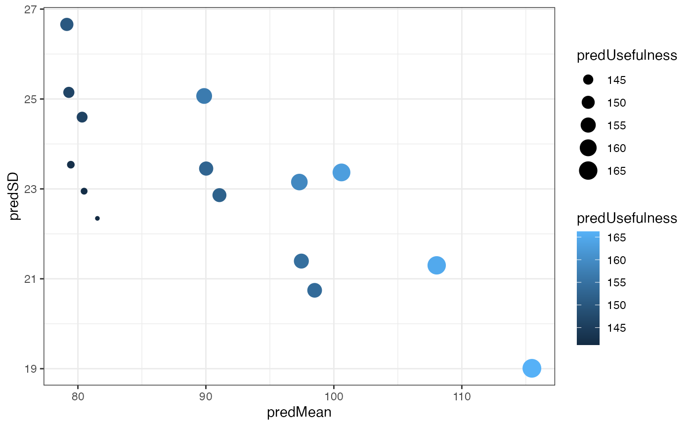
crossPreds$tidyPreds[[1]] %>%
  dplyr::filter(Trait=="SELIND") %>%
  dplyr::slice_max(order_by = predUsefulness, n = 5)
#> # A tibble: 5 × 9
#>   sireID damID Nsegsnps predOf Trait  predMean predVar predSD predUsefulness
#>   <chr>  <chr>    <int> <chr>  <chr>     <dbl>   <dbl>  <dbl>          <dbl>
#> 1 49     49          22 BV     SELIND    115.     361.   19.0           166.
#> 2 49     153         46 BV     SELIND    108.     454.   21.3           165.
#> 3 153    153         33 BV     SELIND    101.     546.   23.4           163.
#> 4 49     228         53 BV     SELIND     97.3    536.   23.2           159.
#> 5 153    228         55 BV     SELIND     89.9    628.   25.1           157.
  # arrange(desc(predUsefulness)) %>% slice(1:5) # same as `slice_max`
Next steps
That concludes the quick demo, focused on input formatting and output contents, using the basic additive-model in the function predictCrosses() to get selection-index cross usefulness predictions.
Additional vignettes
In subsequent vignettes I will provide:
- Learn the features for incorporating non-additive effects into predictions:
modelType="AD",modelType="DirDomand their correct useage. Includes a theoretical introduction, followed by a demonstration of the use ofrunGenomicPredictions()andpredictCrosses()to accomplish predictions of individual and cross performances.
- Use of the functions for cross-validation (
runCrossVal(),runParentWiseCrossVal(), - possibly the imputation and breeding data processing helper functions (wrappers for e.g. Beagle and code for BreedBase data cleaning).