14 Accuracy of cross prediction?
Context and Purpose:
Upstream: Section @ref() -
Downstream:
Inputs:
Expected outputs:
Before proceeding, one note: the steps below may be hard for some breeding programs, especially when open-pollination is used, most families are small, both parents are not genotyped. If this is the case, or your attempt to implement the steps below fail, do not despair. The k-fold cross-validation accuracy should (hopefully) be related to the accuracy of predicting cross-variances. Therefore, these steps are not 100% necessary for implementing mate selection. Furthermore, mate selection can be done simply on the basis of predicted family-means, whose prediction accuracy should definitely be forecast based on the k-fold cross-validation accuracy. Predicting the usefulness of crosses (remember \(\hat{UC} = \hat{\mu} + i \times \hat{\sigma}\)) requires the prediction of cross-variance (the \(\hat{\sigma}\) part), which requires accurate phasing information for non-inbred lines.
14.1 Pedigree
We downloaded a pedigree in the last section of the “download training data” chapter.
14.1.1 Read pedigree
# read.table() throws an error, some aspect of the formatting from the database download
## read.table(here::here("data","pedigree.txt"),
##            stringsAsFactors = F, header = T)

# use read_delim instead
ped<-read_delim(here::here("data","pedigree.txt"),delim = "\t")
#> Rows: 963 Columns: 4
#> ── Column specification ────────────────────────────────────
#> Delimiter: "\t"
#> chr (4): Accession, Female_Parent, Male_Parent, Cross_Type
#>
#> ℹ Use `spec()` to retrieve the full column specification for this data.
#> ℹ Specify the column types or set `show_col_types = FALSE` to quiet this message.
Filter: Keep only complete pedigree records.
ped %<>%
     dplyr::select(-Cross_Type) %>%
     filter(!is.na(Female_Parent),
            !is.na(Male_Parent),
            Female_Parent!="?",
            Male_Parent!="?") %>%
     distinct
Number of full-sib families?
462 in this set.
Summarize distribution of full-sib family sizes
ped %>%
  count(Female_Parent,Male_Parent) %>% arrange(desc(n))  %>%  summary(.$n)
#>  Female_Parent      Male_Parent              n
#>  Length:462         Length:462         Min.   :1.000
#>  Class :character   Class :character   1st Qu.:1.000
#>  Mode  :character   Mode  :character   Median :1.000
#>                                        Mean   :1.294
#>                                        3rd Qu.:1.000
#>                                        Max.   :7.000
Less than 1/3 families have more than 1 member. We need >>2 members for this analysis.
14.1.2 Fully genotyped trios?
For the parent-wise cross-validation, we need pedigree entrees where not both of the 2 parents and the accession itself are in our genotyped dataset. We don’t need them to necessarily be phenotyped though.
Are all of the entrees themselves genotyped?
Yes. That was pretty much assured by the way we set-up the download originally.
There is no guarantee on the parents though…
Indeed, only portions of the parents are present in our SNP data.
genotyped_ped<-ped %>%
     filter(Accession %in% genotyped_gids,
            Female_Parent %in% genotyped_gids,
            Male_Parent %in% genotyped_gids)
genotyped_ped %>% nrow()
#> [1] 135
That leaves us with a very small set of complete trios (accession + male parent + female parent).
genotyped_ped %>%
     count(Female_Parent,Male_Parent) %>% arrange(desc(n))  %>%  summary(.$n)
#>  Female_Parent      Male_Parent              n
#>  Length:104         Length:104         Min.   :1.000
#>  Class :character   Class :character   1st Qu.:1.000
#>  Mode  :character   Mode  :character   Median :1.000
#>                                        Mean   :1.298
#>                                        3rd Qu.:1.000
#>                                        Max.   :7.000
Looks like 104 full-sib families.
How many families have >1 offspring?
genotyped_ped %>%
     count(Female_Parent,Male_Parent) %>%
     filter(n>1)
#> # A tibble: 18 × 3
#>    Female_Parent        Male_Parent             n
#>    <chr>                <chr>               <int>
#>  1 IITA-TMS-IBA011371   IITA-TMS-IBA011371      4
#>  2 IITA-TMS-IBA020431   IITA-TMS-IBA030055A     2
#>  3 IITA-TMS-IBA030060   IITA-TMS-IBA010903      2
#>  4 IITA-TMS-IBA030060   IITA-TMS-MM970043       3
#>  5 IITA-TMS-IBA30555    TMEB1                   2
#>  6 IITA-TMS-IBA4(2)1425 TMEB1                   2
#>  7 IITA-TMS-IBA8902195  IITA-TMS-IBA950379      2
#>  8 IITA-TMS-IBA9001554  IITA-TMS-IBA011659      2
#>  9 IITA-TMS-IBA91934    TMEB1                   7
#> 10 IITA-TMS-IBA940330   IITA-TMS-IBA011224      3
#> 11 IITA-TMS-IBA961089A  IITA-TMS-IBA961089A     2
#> 12 IITA-TMS-IBA961632   IITA-TMS-IBA000070      2
#> 13 IITA-TMS-IBA961632   IITA-TMS-IBA030055A     3
#> 14 IITA-TMS-IBA972205   TMEB1937                5
#> 15 IITA-TMS-ZAR930151   IITA-TMS-MM970043       2
#> 16 TMS13F1307P0004      TMS13F1343P0044         2
#> 17 TMS14F1016P0006      TMS14F1035P0004         2
#> 18 TMS14F1255P0005      TMS13F1343P0044         2
In the end, our small example dataset has only 18 families with >1 offspring.
Remember that: (1) This is a small, example dataset, and (2) our goal is to estimate the accuracy of predicting the genetic-variance in a family.
For reference sake: In a previous analysis for IITA’s large training population, I had ~6200 entries in the pedigree, 196 full-sib families with >=10 members, and the average family size was ~5.
It is unlikely this is sufficient for a good estimate, it’s possible this won’t even work in the analysis, but we will try!
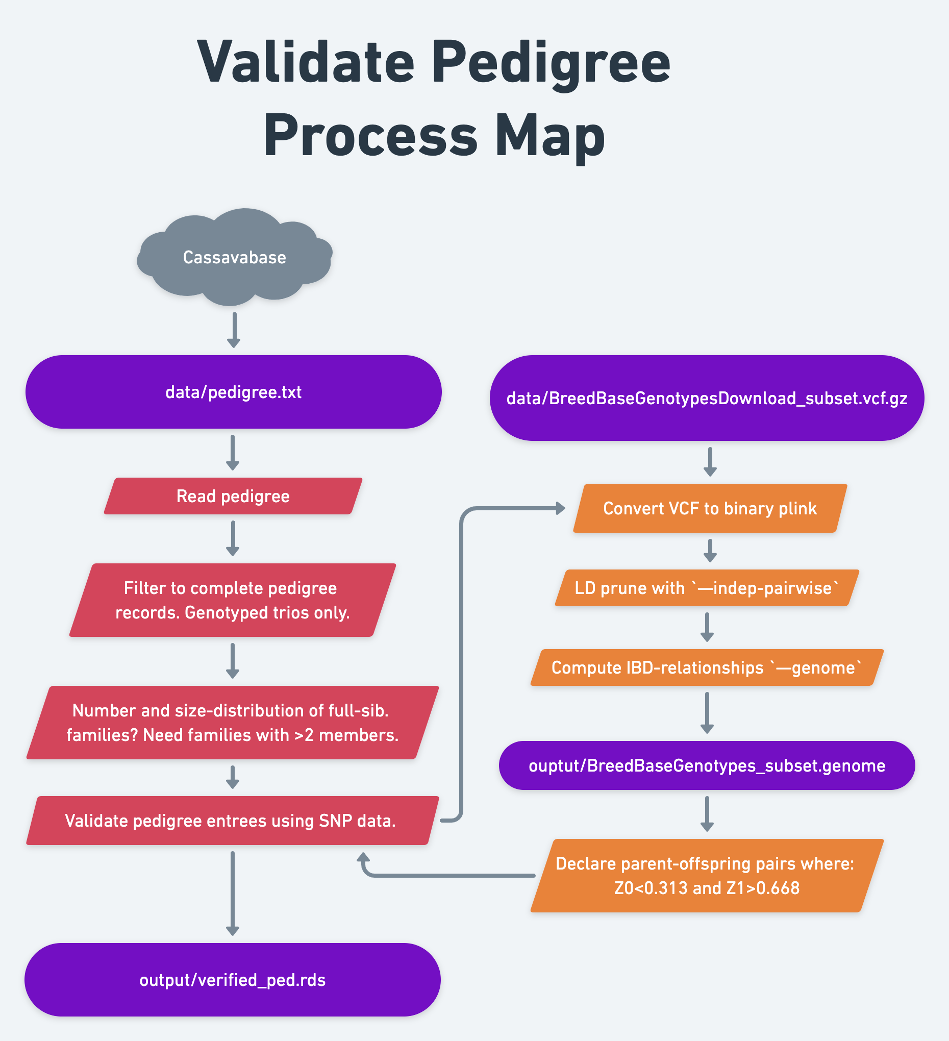
14.2 Verify pedigree relationships
There is one additional step I highly recommend and will demonstrate here.
Plant breeding pedigrees can often have errors, esp. for the male (pollen) parent. For that reason, I recommend using the genomic data to check the pedigree. We do not want our estimate of family-genetic variance prediction accuracy further detrimated by the presence of incorrect pedigree entrees.
There are various software options to do this, probably an R package or two.
My approach uses the --genome IBD calculator in the command-line program PLINK v1.9, click here for the PLINK1.9 manual and to download/install the program.
See an example implementation done in 2021 here: https://wolfemd.github.io/IITA_2021GS/03-validatePedigree.html
PLINK1.9 pipeline to use:
Convert the VCF file to binary plink format
-
For a full dataset / “official anlaysis”:
- 2a: Subset whole-pop. binary plink files to only lines in the pedigree.
- 2b: LD-prune
--indep-pairwise 100 25 0.25stringent, but somewhat arbitrary - Skip this step in the example dataset: population is small and we already randomly sampled a small number of markers to make compute faster in the example meaning that LD is probably low.
Compute IBD-relationships
--genomeParent-offspring relationships determination (see below)
Determine parent-offspring relationship status based on plink IBD:
should have a kinship \(\hat{\pi} \approx 0.5\).
Three standard IBD probabilities are defined for each pair; the probability of sharing zero (Z0), one (Z1) or two (Z2) alleles at a randomly chosen locus IBD.
The expectation for siblings in terms of these probabilities is Z0=0.25, Z1=0.5 and Z2=0.25.
The expectation for parent-offspring pairs is Z0=0, Z1=1 and Z2=0.
Based on work I did in 2016 (never published), declare a parent-offspring pair where: Z0<0.313 and Z1>0.668.
14.2.2 Install plink1.9 (Mac)
Your results will vary. Here is how I got it installed on my mac laptop.
- Downloaded it to my
~/Downloads/folder and unzipped (double-click the .zip file) - At the terminal:
cd ~/Downloads/plink_mac_20220305 - Move the binary file (
plink) to my command-line path:cp ~/Downloads/plink_mac_20220305/plink /usr/local/bin/ - Now typing
plinkat the command line will always engage the program - However, I had to convince MacOS that it was safe by following this instruction: https://zaiste.net/os/macos/howtos/resolve-macos-cannot-be-opened-because-the-developer-cannot-be-verified-error/
14.2.3 Make binary plink from VCF
# in the terminal change directory
# go to the data/ directory where the VCF file is located
plink --vcf BreedBaseGenotypes_subset.vcf.gz \
     --make-bed --const-fid --keep-allele-order \
     --out BreedBaseGenotypes_subset
14.2.4 Run plink IBD
plink --bfile BreedBaseGenotypes_subset \
  --genome \
  --out ../output/BreedBaseGenotypes_subset;
This creates an output file with extension *.genome in the output directory. For our 963 individual dataset, the file size is only 60M… beware, it could get huge if you have many samples.
See the plink1.9 manual here: https://www.cog-genomics.org/plink/1.9/ibd for details on what this does and what the output means.
14.2.5 Verify parent-offspring relationships
genome<-read.table(here::here("output/","BreedBaseGenotypes_subset.genome"),
                   stringsAsFactors = F,header = T) %>%
     as_tibble
genome %>% head
#> # A tibble: 6 × 14
#>    FID1 IID1     FID2 IID2    RT       EZ    Z0     Z1    Z2
#>   <int> <chr>   <int> <chr>   <chr> <int> <dbl>  <dbl> <dbl>
#> 1     0 IITA-T…     0 IITA-T… OT        0 0.616 0.384  0
#> 2     0 IITA-T…     0 IITA-T… OT        0 0.663 0.337  0
#> 3     0 IITA-T…     0 IITA-T… OT        0 0.607 0.283  0.110
#> 4     0 IITA-T…     0 IITA-T… OT        0 0     0.0612 0.939
#> 5     0 IITA-T…     0 IITA-T… OT        0 0     0.0526 0.947
#> 6     0 IITA-T…     0 IITA-T… OT        0 0     1      0
#> # … with 5 more variables: PI_HAT <dbl>, PHE <int>,
#> #   DST <dbl>, PPC <dbl>, RATIO <dbl>
dim(genome)
#> [1] 463203     14
ped %>%
     semi_join(genome %>% rename(Accession=IID1,Female_Parent=IID2)) %>%
     left_join(genome %>% rename(Accession=IID1,Female_Parent=IID2))
#> Joining, by = c("Accession", "Female_Parent")
#> Joining, by = c("Accession", "Female_Parent")
#> # A tibble: 4 × 15
#>   Accession   Female_Parent   Male_Parent   FID1  FID2 RT
#>   <chr>       <chr>           <chr>        <int> <int> <chr>
#> 1 IITA-TMS-B… TMEB1           IITA-TMS-IB…     0     0 OT
#> 2 IITA-TMS-I… IITA-TMS-IBA90… IITA-TMS-IB…     0     0 OT
#> 3 IITA-TMS-I… TMEB1           IITA-TMS-IB…     0     0 OT
#> 4 IITA-TMS-I… IITA-TMS-IBA91… IITA-TMS-IB…     0     0 OT
#> # … with 9 more variables: EZ <int>, Z0 <dbl>, Z1 <dbl>,
#> #   Z2 <dbl>, PI_HAT <dbl>, PHE <int>, DST <dbl>,
#> #   PPC <dbl>, RATIO <dbl>
# Confirm Female_Parent - Offspring Relationship
## In the plink genome file
## IID1 or IID2 could be the Accession or the Female_Parent
conf_female_ped<-genotyped_ped %>%
     inner_join(genome %>%
                     rename(Accession=IID1,Female_Parent=IID2)) %>%
     bind_rows(genotyped_ped %>%
                    inner_join(genome %>%
                                    rename(Accession=IID2,Female_Parent=IID1))) %>%
     # Declare confirm-reject Accession-Female_Parent
     mutate(ConfirmFemaleParent=case_when(Z0<0.32 & Z1>0.67~"Confirm",
                                          # Relatedness coeff differ if the Accession is the result of a self-cross
                                          Male_Parent==Female_Parent & PI_HAT>0.6 & Z0<0.3 & Z2>0.32~"Confirm",
                                          TRUE~"Reject")) %>%
     dplyr::select(Accession,Female_Parent,ConfirmFemaleParent)
#> Joining, by = c("Accession", "Female_Parent")
#> Joining, by = c("Accession", "Female_Parent")
## Now do the same for the Accession-Male_Parent relationships
conf_male_ped<-genotyped_ped %>%
     inner_join(genome %>%
                     rename(Accession=IID1,Male_Parent=IID2)) %>%
     bind_rows(genotyped_ped %>%
                    inner_join(genome %>%
                                    rename(Accession=IID2,Male_Parent=IID1))) %>%
     # Declare confirm-reject Accession-Female_Parent
     mutate(ConfirmMaleParent=case_when(Z0<0.32 & Z1>0.67~"Confirm",
                                          # Relatedness coeff differ if the Accession is the result of a self-cross
                                          Male_Parent==Female_Parent & PI_HAT>0.6 & Z0<0.3 & Z2>0.32~"Confirm",
                                          TRUE~"Reject")) %>%
     dplyr::select(Accession,Male_Parent,ConfirmMaleParent)
#> Joining, by = c("Accession", "Male_Parent")
#> Joining, by = c("Accession", "Male_Parent")
# Now join the confirmed female and male relationships
# This regenerates the original "genotyped_ped" with two added columns
confirmed_ped<-conf_female_ped %>%
     left_join(conf_male_ped) %>%
     relocate(Male_Parent,.before = "ConfirmFemaleParent")
#> Joining, by = "Accession"
So, how well supported are the pedigree relationships according to my approach?
confirmed_ped %>%
     count(ConfirmFemaleParent,ConfirmMaleParent) %>%
     mutate(Prop=round(n/sum(n),2))
#> # A tibble: 4 × 4
#>   ConfirmFemaleParent ConfirmMaleParent     n  Prop
#>   <chr>               <chr>             <int> <dbl>
#> 1 Confirm             Confirm             105  0.78
#> 2 Confirm             Reject               10  0.07
#> 3 Reject              Confirm               5  0.04
#> 4 Reject Reject 15 0.11- 78% of Accessions had both parents correct.
- 7% had the female but not the male correct.
- 4% had the male but not the female
14.2.6 Subset to fully-validated trios
We can only run the cross-validation using a pedigree where the full trio (Accession’s relationship to both parents) is validated.
Remove any without both parents confirmed.
valid_ped<-confirmed_ped %>%
     filter(ConfirmFemaleParent=="Confirm",
         ConfirmMaleParent=="Confirm") %>%
dplyr::select(-contains("Confirm"))Leaves us with 105 validated entries in the pedigree
valid_ped %>%
     count(Female_Parent,Male_Parent) %>%
     filter(n>1)
#> # A tibble: 16 × 3
#>    Female_Parent        Male_Parent             n
#>    <chr>                <chr>               <int>
#>  1 IITA-TMS-IBA011371   IITA-TMS-IBA011371      4
#>  2 IITA-TMS-IBA020431   IITA-TMS-IBA030055A     2
#>  3 IITA-TMS-IBA030060   IITA-TMS-IBA010903      2
#>  4 IITA-TMS-IBA030060   IITA-TMS-MM970043       3
#>  5 IITA-TMS-IBA4(2)1425 TMEB1                   2
#>  6 IITA-TMS-IBA8902195  IITA-TMS-IBA950379      2
#>  7 IITA-TMS-IBA9001554  IITA-TMS-IBA011659      2
#>  8 IITA-TMS-IBA91934    TMEB1                   6
#>  9 IITA-TMS-IBA961089A  IITA-TMS-IBA961089A     2
#> 10 IITA-TMS-IBA961632   IITA-TMS-IBA000070      2
#> 11 IITA-TMS-IBA961632   IITA-TMS-IBA030055A     3
#> 12 IITA-TMS-IBA972205   TMEB1937                5
#> 13 IITA-TMS-ZAR930151   IITA-TMS-MM970043       2
#> 14 TMS13F1307P0004      TMS13F1343P0044         2
#> 15 TMS14F1016P0006      TMS14F1035P0004         2
#> 16 TMS14F1255P0005      TMS13F1343P0044         2
Luckily, 16 of the 18 full-sib families that have >1 entry are still here.
valid_ped %>%
     count(Female_Parent,Male_Parent) %>%
     filter(n>2)
#> # A tibble: 5 × 3
#>   Female_Parent      Male_Parent             n
#>   <chr>              <chr>               <int>
#> 1 IITA-TMS-IBA011371 IITA-TMS-IBA011371      4
#> 2 IITA-TMS-IBA030060 IITA-TMS-MM970043       3
#> 3 IITA-TMS-IBA91934  TMEB1                   6
#> 4 IITA-TMS-IBA961632 IITA-TMS-IBA030055A     3
#> 5 IITA-TMS-IBA972205 TMEB1937                5
Though only 5 families have more than 2…
14.3 Parent-wise cross-validation
Refer to the following:
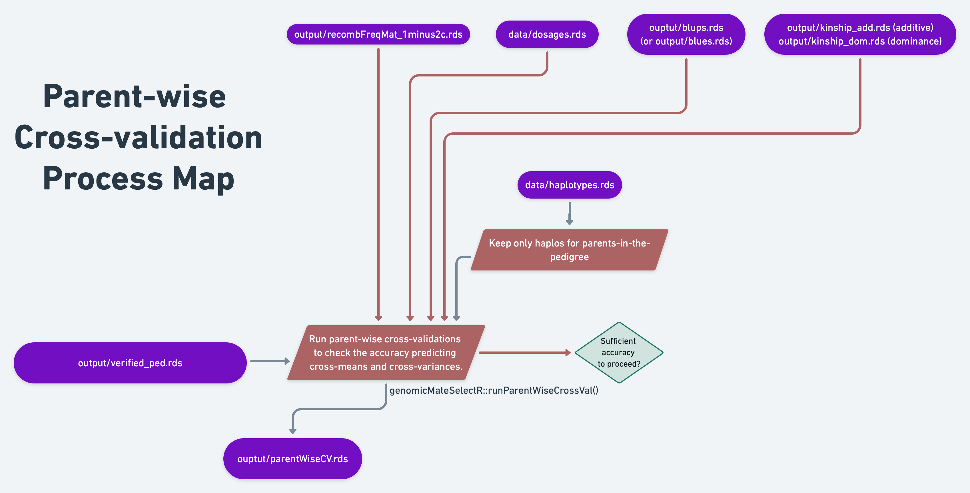
14.3.2 Load inputs and set-up
# Load verified ped
ped<-readRDS(here::here("output","verified_ped.rds")) %>%
     # Rename things to match genomicMateSelectR::runParentWiseCrossVal()
     rename(GID=Accession,
            sireID=Male_Parent,
            damID=Female_Parent)
# Keep only families with _at least_ 2 offspring
ped %<>%
     semi_join(ped %>% count(sireID,damID) %>% filter(n>1) %>% ungroup())

# GENOMIC RELATIONSHIP MATRIX
grms<-list(A=readRDS(file=here::here("output","kinship_add.rds")))

# BLUPs
blups<-readRDS(here::here("output","blups.rds")) %>%
     # based on cross-validation, decided to exclude MCMDS from this analysis
     filter(Trait != "MCMDS") %>%
     # need to rename the "blups" list to comply with the runCrossVal function
     rename(TrainingData=blups) %>%
     dplyr::select(Trait,TrainingData) %>%
     # need also to remove phenotyped-but-not-genotyped lines
     mutate(TrainingData=map(TrainingData,
                             ~filter(.,germplasmName %in% rownames(grms$A)) %>%
                                  # rename the germplasmName column to GID
                                  rename(GID=germplasmName))) %>%
     # It seems actually that runParentWiseCrossVal() wnats this column named "blups"
     rename(blups=TrainingData)

# DOSAGE MATRIX
## Dosages are also needed inside the runParentWiseCrossVal() function
## Reason is that they are used to extra SNP effects from GBLUP models
dosages<-readRDS(here::here("data","dosages.rds"))

# HAPLOTYPE MATRIX
## keep only haplos for parents-in-the-pedigree
## those which will be used in prediction, saves memory
haploMat<-readRDS(file=here::here("data","haplotypes.rds"))
parents<-union(ped$sireID,ped$damID)
parenthaps<-sort(c(paste0(parents,"_HapA"),
                   paste0(parents,"_HapB")))
haploMat<-haploMat[parenthaps,]

# SELECTION INDEX
SIwts<-c(DM=15,
         logFYLD=20,
         logDYLD=20)
In the genotype data processing stage, specifically in one of the last steps, we created a recombination frequency matrix. To do this, we accessed a genetic map, interpolated it to the markers in our dataset and then used helper functions provided by genomicMateSelectR. We finally need that matrix.
14.3.3 Run cross-validation
starttime<-proc.time()[3]
parentWiseCV<-runParentWiseCrossVal(nrepeats=2,nfolds=5,seed=121212,
                                    modelType="A",
                                    ncores=10,
                                    ped=ped,
                                    blups=blups,
                                    dosages=dosages,
                                    haploMat=haploMat,
                                    grms=grms,
                                    recombFreqMat = recombFreqMat,
                                    selInd = TRUE, SIwts = SIwts)
elapsed<-proc.time()[3]-starttime; elapsed/60
Took about 3.5 minutes using 10 cores on my 16 core - 64 GB RAM machine. Memory usagage wasn’t bad.
14.3.5 Plot results
You will find the output of runParentWiseCrossVal is a list with two elements: “meanPredAccuracy” and “varPredAccuracy”
Take a peak at both to see how it’s formatted:
parentWiseCV$meanPredAccuracy %>% head
#> # A tibble: 6 × 7
#>   Repeat  Fold  modelType predOf Trait predVSobs AccuracyEst
#>   <chr>   <chr> <chr>     <chr>  <chr> <list>          <dbl>
#> 1 Repeat1 Fold1 A         MeanBV SELI… <tibble …      -0.229
#> 2 Repeat1 Fold1 A         MeanBV DM    <tibble …      -0.385
#> 3 Repeat1 Fold1 A         MeanBV logD… <tibble …     NaN
#> 4 Repeat1 Fold1 A         MeanBV logF… <tibble …      -0.771
#> 5 Repeat1 Fold2 A         MeanBV SELI… <tibble …     NaN
#> 6 Repeat1 Fold2 A         MeanBV DM    <tibble …     NaN
parentWiseCV$varPredAccuracy %>% head
#> # A tibble: 6 × 8
#>   Repeat  Fold  modelType predOf Trait1  Trait2  predVSobs
#>   <chr>   <chr> <chr>     <chr>  <chr>   <chr>   <list>
#> 1 Repeat1 Fold1 A         VarBV  SELIND  SELIND  <tibble [6…
#> 2 Repeat1 Fold1 A         VarBV  DM      DM      <tibble [6…
#> 3 Repeat1 Fold1 A         VarBV  DM      logDYLD <tibble [6…
#> 4 Repeat1 Fold1 A         VarBV  DM      logFYLD <tibble [6…
#> 5 Repeat1 Fold1 A         VarBV  logDYLD logDYLD <tibble [6…
#> 6 Repeat1 Fold1 A         VarBV  logDYLD logFYLD <tibble [6…
#> # … with 1 more variable: AccuracyEst <dbl>
parentWiseCV$meanPredAccuracy %>%
     ggplot(.,aes(x=Trait,y=AccuracyEst,fill=Trait)) + geom_boxplot() +
     labs(title="Accuracy Predicting Family Means")
#> Warning: Removed 29 rows containing non-finite values
#> (stat_boxplot).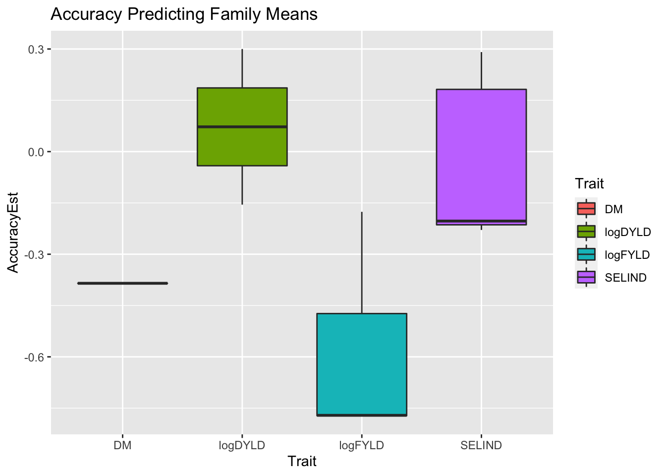
Obviously not a good result, must have to do with the tiny dataset both for training prediction models (to get marker effects) and in terms of the small number of family-members in the small number of families available.
parentWiseCV$varPredAccuracy %>%
     # this will format the two column information
     # indicating variances and covariances
     # into a single variable for the plot
     mutate(VarParam=paste0(Trait1,"\n",Trait2)) %>%
     ggplot(.,aes(x=VarParam,y=AccuracyEst,fill=VarParam)) + geom_boxplot()
#> Warning: Removed 57 rows containing non-finite values
#> (stat_boxplot).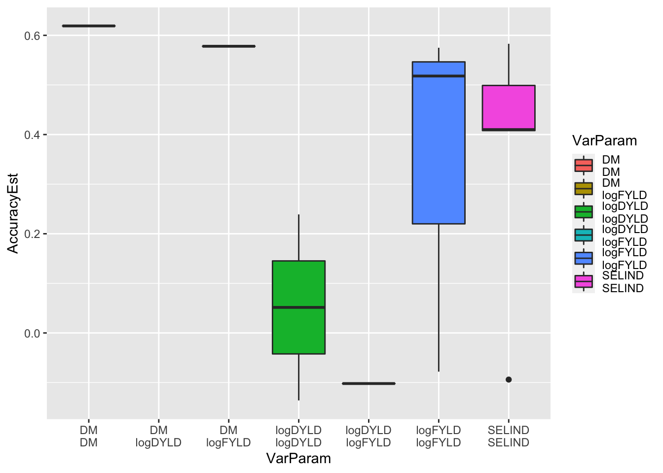
Surprising the variance accuracy actually appears much better than the mean accuracy… should definitely take this with equal skepticism to the result for the mean, for the same reasons!