7 Prepare phenotype data
- Context and Purpose: In this step, we do quality control, clean and format training data for further analysis.
- Upstream: Section 6 - training data download
- Downstream: pretty much everything
- Inputs: “Raw” field trial data
- Expected outputs: “Cleaned” field trial data
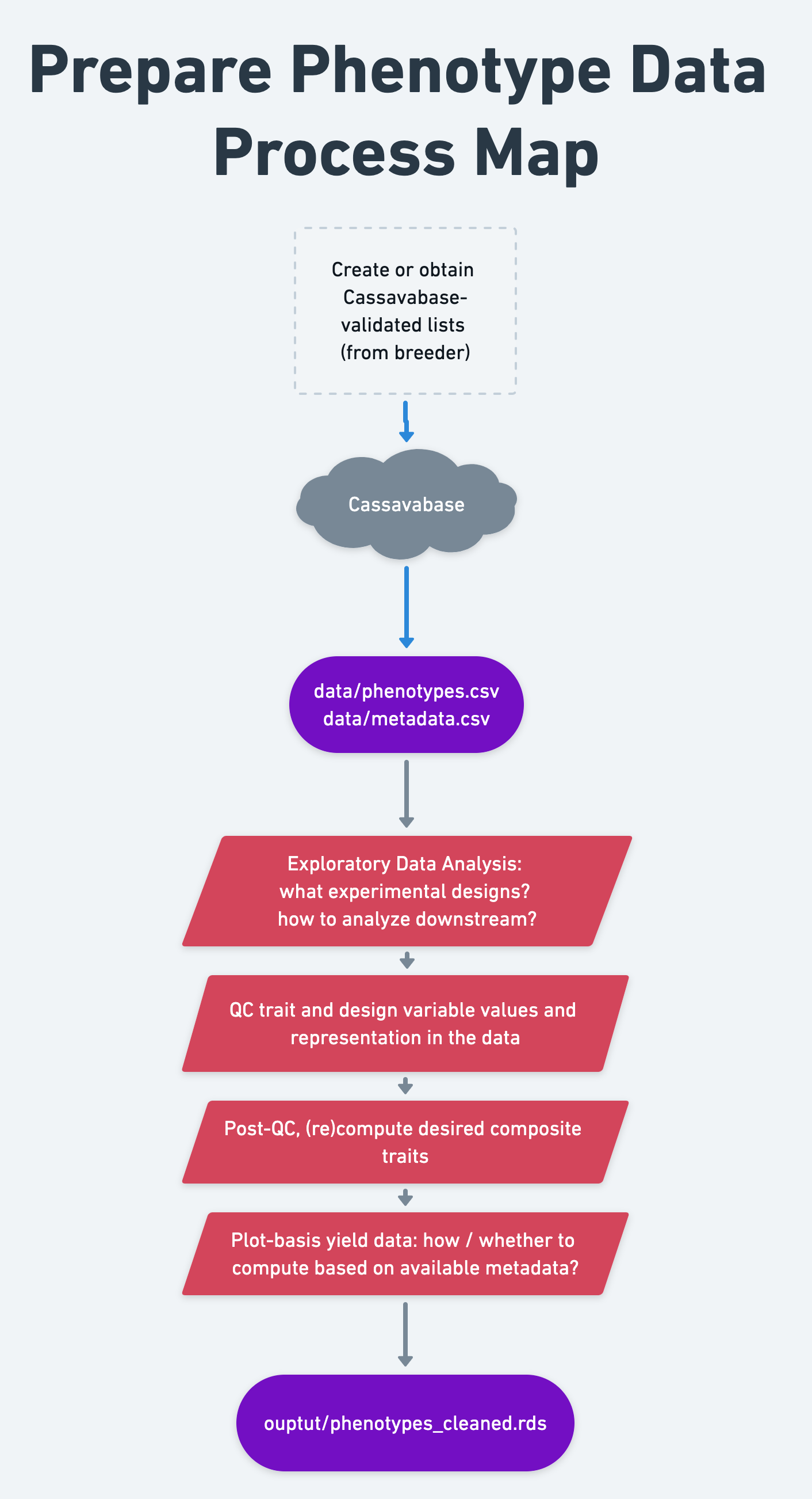
7.2 Read DB data
Load the phenotype and metadata downloads into R.
I built a function readDBdata that simply wraps around read.csv, reads and merges the metadata to the plot-basis data. The metadataFile= argument can be left NULL.
dbdata<-readDBdata(phenotypeFile = here::here("data","phenotype.csv"),
                   metadataFile = here::here("data","metadata.csv"))
#> Joining, by = c("studyYear", "programDbId", "programName", "programDescription", "studyDbId", "studyName", "studyDescription", "studyDesign", "plotWidth", "plotLength", "fieldSize", "fieldTrialIsPlannedToBeGenotyped", "fieldTrialIsPlannedToCross", "plantingDate", "harvestDate", "locationDbId", "locationName")
HINT: At any point in the manual, if I reference or use a custom function in the genomicMateSelectR, I encourage you to check out the reference page for that function, e.g. readDBdata(). Or look at the code yourself by typing e.g. readDBdata at the R console or heading to the GitHub repo.
7.3 Check experimental designs
Checklist: Are the data plot-basis, plant-basis or a mixture? If plant-basis data are present, should they be converted to plot-basis for further analysis?
dbdata %>% count(observationLevel)
#>   observationLevel    n
#> 1             plot 2533
# table(dbdata$observationLevel)
Only plot-basis in this case.
Checklist: What experimental designs are present? How are they represented by the variables in the dataset? Are all designs consistent with your expectations, for example relative to the reported “trialType,” “studyName” and/or “studyDesign?”
In this step, in the past, I have not been certain of the experimental designs of the trials I had downloaded. I was also not certain how the designs were represented in the column-names. For this reason, I developed an ad hoc custom code to “detect” the designs. I built the genomicMateSelectR function detectExptDesigns(). See an example here.
RECOMMENDATION: Each analyst needs to use exploratory data anlaysis, making summary statistics and plots as necessary to determine how the data should be modelled downstream. If there are missing or incorrectly represented trial design variables, get it corrected on the database (contact breeding program data manager, as necessary).
Because I have a small example dataset, it is possible to look at 9 trials and evaluate.
Often, many more trials are part of a genomic prediction. This is why it is essential that trial designs be consistent, and clear to the analyst. You may need to derive a strategy similar to the detectExptDesigns() function to semi-automate the process.
library(gt)
dbdata %>%
     count(studyName,trialType, studyDesign, numberBlocks,numberReps,entryType) %>%
     spread(entryType,n) %>%
     gt()  %>%
tab_options(table.font.size = pct(75))| studyName | trialType | studyDesign | numberBlocks | numberReps | check | test |
|---|---|---|---|---|---|---|
| 19.GS.C1.C2.C3.AYT.42.UB | NA | Alpha | NA | NA | 15 | 110 |
| 19.GS.C2.UYT.36.setA.IB | Uniform Yield Trial | Alpha | 6 | 2 | 10 | 58 |
| 19.GS.C2.UYT.36.setA.UB | Uniform Yield Trial | Alpha | 6 | 2 | 10 | 62 |
| 19.GS.C2.UYT.36.setB.IB | Uniform Yield Trial | RCBD | 6 | 2 | 10 | 56 |
| 19.GS.C2.UYT.36.setB.UB | Uniform Yield Trial | Alpha | 6 | 2 | 10 | 62 |
| 19.GS.C4B.PYT.135.UB | Preliminary Yield Trial | Alpha | 30 | 2 | 12 | 258 |
| 19.GS.C4B.PYT.140.IB | Preliminary Yield Trial | Alpha | 28 | 2 | 31 | 242 |
| 19.GS.C4C.CE.822.IB | Clonal Evaluation | RCBD | 42 | 1 | 132 | 645 |
| 19geneticgainUB | genetic_gain_trial | Augmented | 11 | 1 | NA | 810 |
Summary table above shows:
- trialType and studyDesign cannot be 100% relied upon, at least not here.
- The only trial actually listed as having
studyDesign=="Augmented"does not have “check” vs. “test” distinguished in the “entryType.” - A
trialType=="Clonal Evaluation"withstudyDesign=="RCBD"but actually only 1 replication.
Next, I’ll check if the replicate and blockNumber columns reliably distinguish complete and incomplete blocks in the data.
dbdata %>%
     group_by(studyName) %>%
     summarize(N_replicate=length(unique(replicate)),
               N_blockNumber=length(unique(blockNumber))) %>%
gt() %>% tab_options(table.font.size = pct(75))| studyName | N_replicate | N_blockNumber |
|---|---|---|
| 19.GS.C1.C2.C3.AYT.42.UB | 3 | 3 |
| 19.GS.C2.UYT.36.setA.IB | 2 | 6 |
| 19.GS.C2.UYT.36.setA.UB | 2 | 6 |
| 19.GS.C2.UYT.36.setB.IB | 2 | 6 |
| 19.GS.C2.UYT.36.setB.UB | 2 | 6 |
| 19.GS.C4B.PYT.135.UB | 2 | 30 |
| 19.GS.C4B.PYT.140.IB | 2 | 28 |
| 19.GS.C4C.CE.822.IB | 1 | 42 |
| 19geneticgainUB | 1 | 11 |
Here, I notice that except 1 trial (19.GS.C1.C2.C3.AYT.42.UB) has the same number of reps and blocks.
The question is, are complete replications of the experiment indicated by replicate and incomplete sub-blocks represented by blockNumber
dbdata %>%
     group_by(studyName) %>%
     summarize(N_replicate=length(unique(replicate)),
               N_blockNumber=length(unique(blockNumber)),
               doRepsEqualBlocks=all(replicate==blockNumber)) %>%
gt() %>% tab_options(table.font.size = pct(75))| studyName | N_replicate | N_blockNumber | doRepsEqualBlocks |
|---|---|---|---|
| 19.GS.C1.C2.C3.AYT.42.UB | 3 | 3 | TRUE |
| 19.GS.C2.UYT.36.setA.IB | 2 | 6 | FALSE |
| 19.GS.C2.UYT.36.setA.UB | 2 | 6 | FALSE |
| 19.GS.C2.UYT.36.setB.IB | 2 | 6 | FALSE |
| 19.GS.C2.UYT.36.setB.UB | 2 | 6 | FALSE |
| 19.GS.C4B.PYT.135.UB | 2 | 30 | FALSE |
| 19.GS.C4B.PYT.140.IB | 2 | 28 | FALSE |
| 19.GS.C4C.CE.822.IB | 1 | 42 | FALSE |
| 19geneticgainUB | 1 | 11 | FALSE |
So for 1 trial, there are 3 complete blocks, no sub-blocks. For 6 trials, there are 2 complete replications and nested sub-blocks represented by the blockNumber variable. For 2 trials, there are only incomplete blocks.
Next, I decided to check that the replicate column definitely means complete blocks. The below might look a bit complicated, but I basically merge two summaries: (1) he overall number of accessions per trial, and (2) the average number of accessions per replicate per trial.
# the overall number of accessions per trial
dbdata %>%
     group_by(studyName) %>%
     summarize(N_accession=length(unique(germplasmName))) %>%
     # the average number of accessions per replicate per trial
     left_join(dbdata %>%
                    group_by(studyName,replicate) %>%
                    summarize(N_accession=length(unique(germplasmName))) %>%
                    group_by(studyName) %>%
                    summarize(avgAccessionsPerReplicate=ceiling(mean(N_accession)))) %>%
     gt() %>% tab_options(table.font.size = pct(75))
#> `summarise()` has grouped output by 'studyName'. You can override using the `.groups` argument.
#> Joining, by = "studyName"| studyName | N_accession | avgAccessionsPerReplicate |
|---|---|---|
| 19.GS.C1.C2.C3.AYT.42.UB | 42 | 42 |
| 19.GS.C2.UYT.36.setA.IB | 35 | 34 |
| 19.GS.C2.UYT.36.setA.UB | 36 | 36 |
| 19.GS.C2.UYT.36.setB.IB | 36 | 33 |
| 19.GS.C2.UYT.36.setB.UB | 36 | 36 |
| 19.GS.C4B.PYT.135.UB | 135 | 135 |
| 19.GS.C4B.PYT.140.IB | 129 | 127 |
| 19.GS.C4C.CE.822.IB | 657 | 657 |
| 19geneticgainUB | 782 | 782 |
The numbers are very similar for all trials, indicating complete blocks.
One more: look at the min, mean and max number of accessions per blockNumber.
# the overall number of accessions per trial
dbdata %>%
     group_by(studyName) %>%
     summarize(N_accession=length(unique(germplasmName))) %>%
     left_join(dbdata %>%
     group_by(studyName,replicate,blockNumber) %>%
     summarize(N_accession=length(unique(germplasmName))) %>% ungroup() %>%
     group_by(studyName) %>%
     summarize(minAccessionsPerBlock=ceiling(min(N_accession)),
               avgAccessionsPerBlock=ceiling(mean(N_accession)),
               maxAccessionsPerBlock=ceiling(max(N_accession)))) %>%
     gt() %>% tab_options(table.font.size = pct(60))
#> `summarise()` has grouped output by 'studyName', 'replicate'. You can override using the `.groups` argument.
#> Joining, by = "studyName"| studyName | N_accession | minAccessionsPerBlock | avgAccessionsPerBlock | maxAccessionsPerBlock |
|---|---|---|---|---|
| 19.GS.C1.C2.C3.AYT.42.UB | 42 | 41 | 42 | 42 |
| 19.GS.C2.UYT.36.setA.IB | 35 | 11 | 12 | 12 |
| 19.GS.C2.UYT.36.setA.UB | 36 | 12 | 12 | 12 |
| 19.GS.C2.UYT.36.setB.IB | 36 | 9 | 11 | 12 |
| 19.GS.C2.UYT.36.setB.UB | 36 | 12 | 12 | 12 |
| 19.GS.C4B.PYT.135.UB | 135 | 9 | 9 | 9 |
| 19.GS.C4B.PYT.140.IB | 129 | 8 | 10 | 10 |
| 19.GS.C4C.CE.822.IB | 657 | 10 | 19 | 20 |
| 19geneticgainUB | 782 | 39 | 73 | 80 |
From this, you can see that except for studyName=="19.GS.C1.C2.C3.AYT.42.UB" the sub-blocks represented by blockNumber have only subsets of the total number of accessions in the trial, as expected.
Further, except for studyName=="19geneticgainUB" all trials have pretty consistently sized sub-blocks.
Now I will ad hoc create two variables (CompleteBlocks and IncompleteBlocks), indicating (TRUE/FALSE) whether to model using the replicate and/or blockNumber variable.
I also like to create explicitly nested design variables (yearInLoc, trialInLocYr, repInTrial, blockInRep).
dbdata %<>%
     group_by(studyName) %>%
     summarize(N_replicate=length(unique(replicate)),
               N_blockNumber=length(unique(blockNumber)),
               doRepsEqualBlocks=all(replicate==blockNumber)) %>%
     ungroup() %>%
     mutate(CompleteBlocks=ifelse(N_replicate>1,TRUE,FALSE),
            IncompleteBlocks=ifelse(N_blockNumber>1 & !doRepsEqualBlocks,TRUE,FALSE)) %>%
     left_join(dbdata) %>%
     mutate(yearInLoc=paste0(programName,"_",locationName,"_",studyYear),
            trialInLocYr=paste0(yearInLoc,"_",studyName),
            repInTrial=paste0(trialInLocYr,"_",replicate),
            blockInRep=paste0(repInTrial,"_",blockNumber))
#> Joining, by = "studyName"
Just to check:
dbdata %>%
     count(studyName,CompleteBlocks,IncompleteBlocks) %>%
     left_join(dbdata %>%
                    group_by(studyName) %>%
                    summarize(nRepInTrial=length(unique(repInTrial)),
                              nBlockInRep=length(unique(blockInRep)))) %>%
     gt() %>% tab_options(table.font.size = pct(67))
#> Joining, by = "studyName"| studyName | CompleteBlocks | IncompleteBlocks | n | nRepInTrial | nBlockInRep |
|---|---|---|---|---|---|
| 19.GS.C1.C2.C3.AYT.42.UB | TRUE | FALSE | 125 | 3 | 3 |
| 19.GS.C2.UYT.36.setA.IB | TRUE | TRUE | 68 | 2 | 6 |
| 19.GS.C2.UYT.36.setA.UB | TRUE | TRUE | 72 | 2 | 6 |
| 19.GS.C2.UYT.36.setB.IB | TRUE | TRUE | 66 | 2 | 6 |
| 19.GS.C2.UYT.36.setB.UB | TRUE | TRUE | 72 | 2 | 6 |
| 19.GS.C4B.PYT.135.UB | TRUE | TRUE | 270 | 2 | 30 |
| 19.GS.C4B.PYT.140.IB | TRUE | TRUE | 273 | 2 | 28 |
| 19.GS.C4C.CE.822.IB | FALSE | TRUE | 777 | 1 | 42 |
| 19geneticgainUB | FALSE | TRUE | 810 | 1 | 11 |
7.4 Traits and Trait Abbreviations
Cassavabase downloads use very long column-names corresponding to the full trait-ontology name. For convenience, I replace these names with abbreviations, documented here. For eventual upload of analysis results, names will need to be restored to ontology terms.
I also use this opportunity to subselect traits.
traitabbrevs<-tribble(~TraitAbbrev,~TraitName,
        "CMD1S","cassava.mosaic.disease.severity.1.month.evaluation.CO_334.0000191",
        "CMD3S","cassava.mosaic.disease.severity.3.month.evaluation.CO_334.0000192",
        "CMD6S","cassava.mosaic.disease.severity.6.month.evaluation.CO_334.0000194",
        "DM","dry.matter.content.percentage.CO_334.0000092",
        "RTWT","fresh.storage.root.weight.per.plot.CO_334.0000012",
        "NOHAV","plant.stands.harvested.counting.CO_334.0000010")
traitabbrevs %>% gt()#rmarkdown::paged_table()| TraitAbbrev | TraitName |
|---|---|
| CMD1S | cassava.mosaic.disease.severity.1.month.evaluation.CO_334.0000191 |
| CMD3S | cassava.mosaic.disease.severity.3.month.evaluation.CO_334.0000192 |
| CMD6S | cassava.mosaic.disease.severity.6.month.evaluation.CO_334.0000194 |
| DM | dry.matter.content.percentage.CO_334.0000092 |
| RTWT | fresh.storage.root.weight.per.plot.CO_334.0000012 |
| NOHAV | plant.stands.harvested.counting.CO_334.0000010 |
Run function renameAndSelectCols() to rename columns and remove unselected traits.
dbdata<-renameAndSelectCols(traitabbrevs,
                            indata=dbdata,
                            customColsToKeep = c("observationUnitName",
                                                 "CompleteBlocks",
                                                 "IncompleteBlocks",
                                                 "yearInLoc",
                                                 "trialInLocYr",
                                                 "repInTrial","blockInRep"))
#> Joining, by = "TraitName"
7.5 QC Trait Values
At this point in the pipeline, we should check the all trait values are in allowable ranges. Different ways to approach this. Feel free to make some plots of your data!
The database also has mechanisms to ensure trait values are only within allowable ranges.
Nevertheless, as a habit, I have an simple ad hoc approach to this:
# comment out the traits not present in this dataset
dbdata<-dbdata %>%
     dplyr::mutate(CMD1S=ifelse(CMD1S<1 | CMD1S>5,NA,CMD1S),
                   CMD3S=ifelse(CMD3S<1 | CMD3S>5,NA,CMD3S),
                   # CMD6S=ifelse(CMD6S<1 | CMD6S>5,NA,CMD6S),
                   # CMD9S=ifelse(CMD9S<1 | CMD9S>5,NA,CMD9S),
                   # CGM=ifelse(CGM<1 | CGM>5,NA,CGM),
                   # CGMS1=ifelse(CGMS1<1 | CGMS1>5,NA,CGMS1),
                   # CGMS2=ifelse(CGMS2<1 | CGMS2>5,NA,CGMS2),
                   DM=ifelse(DM>100 | DM<=0,NA,DM),
                   RTWT=ifelse(RTWT==0 | NOHAV==0 | is.na(NOHAV),NA,RTWT),
                   # SHTWT=ifelse(SHTWT==0 | NOHAV==0 | is.na(NOHAV),NA,SHTWT),
                   # RTNO=ifelse(RTNO==0 | NOHAV==0 | is.na(NOHAV),NA,RTNO),
                   NOHAV=ifelse(NOHAV==0,NA,NOHAV),
                   NOHAV=ifelse(NOHAV>42,NA,NOHAV)
                   # RTNO=ifelse(!RTNO %in% 1:10000,NA,RTNO)
     )
7.6 Post-QC: composite traits
Now that component traits are QC’d, it’s time to compute any composite traits.
By composite traits, I mean traits computed from combinations of other traits.
Examples for cassava: season-wide mean disease severity, harvest index, and fresh root yield.
7.6.1 Season-wide mean disease severity
# [NEW AS OF APRIL 2021]
## VERSION with vs. without CBSD
## Impervious to particular timepoints between 1, 3, 6 and 9 scores

# Without CBSD (West Africa)
dbdata<-dbdata %>%
  mutate(MCMDS=rowMeans(.[,colnames(.) %in% c("CMD1S","CMD3S","CMD6S","CMD9S")], na.rm = T)) %>%
  select(-any_of(c("CMD1S","CMD3S","CMD6S","CMD9S")))

# With CBSD (East Africa)
# dbdata<-dbdata %>%
#   mutate(MCMDS=rowMeans(.[,colnames(.) %in% c("CMD1S","CMD3S","CMD6S","CMD9S")], na.rm = T),
#          MCBSDS=rowMeans(.[,colnames(.) %in% c("CBSD1S","CBSD3S","CBSD6S","CBSD9S")], na.rm = T)) %>%
#   select(-any_of(c("CMD1S","CMD3S","CMD6S","CMD9S","CBSD1S","CBSD3S","CBSD6S","CBSD9S")))
7.6.2 Fresh root yield (FYLD)
RTWT (fresh root weight per plot in kg) –> FYLD (fresh root yield in tons per hectare)
\[FYLD = \frac{RTWT_{kg / plot}}{MaxHarvestedPlantsPerPlot \times PlantSpacing}\times10\] NOTE: MaxHarvestedPlantsPerPlot in formula above is to distinguish from the plantsPerPlot meta-data field, in case that a net-plot harvest is used. In other words, the value should be the total number of plants intended for harvest in a plot, assuming there were no missing plants in the plot.
PlantSpacing is the area in \(m^2\) per plant.
dbdata %>%
     count(studyYear,studyName,studyDesign,plotWidth,plotLength,plantsPerPlot) %>%
     mutate(plotArea=plotWidth*plotLength) %>%
gt() %>% tab_options(table.font.size = pct(67))| studyYear | studyName | studyDesign | plotWidth | plotLength | plantsPerPlot | n | plotArea |
|---|---|---|---|---|---|---|---|
| 2019 | 19.GS.C1.C2.C3.AYT.42.UB | Alpha | 4 | 4.0 | NA | 125 | 16.0 |
| 2019 | 19.GS.C2.UYT.36.setA.IB | Alpha | 4 | 4.0 | NA | 68 | 16.0 |
| 2019 | 19.GS.C2.UYT.36.setA.UB | Alpha | 4 | 4.0 | NA | 72 | 16.0 |
| 2019 | 19.GS.C2.UYT.36.setB.IB | RCBD | 4 | 4.0 | NA | 66 | 16.0 |
| 2019 | 19.GS.C2.UYT.36.setB.UB | Alpha | 4 | 4.0 | NA | 72 | 16.0 |
| 2019 | 19.GS.C4B.PYT.135.UB | Alpha | 2 | 4.0 | NA | 270 | 8.0 |
| 2019 | 19.GS.C4B.PYT.140.IB | Alpha | 3 | 2.5 | NA | 273 | 7.5 |
| 2019 | 19.GS.C4C.CE.822.IB | RCBD | 1 | 2.5 | NA | 777 | 2.5 |
| 2019 | 19geneticgainUB | Augmented | 1 | 2.5 | NA | 810 | 2.5 |
In the example trial data, the plantsPerPlot meta-data field is empty. To my knowledge, no meta-data field is available in BreedBase to represent a net-plot harvest.
RECOMMEND INPUTING plantsPerPlot meta-data to cassavabase for your breeding program!
Luckily, since there are only 9 trials and this is a tutorial, we will decisions manually.
Firstly noting that the trial 19geneticgainUB actually does not have phenotypes (for any trait). It will be excluded downstream. (I might find a substitute genetic gain trial, from an earlier year, for the sake of this example)
To decide what the real MaxHarvestedPlantsPerPlot and plantsPerPlot were likely to have been, I make two plots below and also compute the maximum NOHAV for each trial.
dbdata %>%
     ggplot(.,aes(x=NOHAV, fill=studyName)) + geom_density(alpha=0.75)
#> Warning: Removed 921 rows containing non-finite values
#> (stat_density).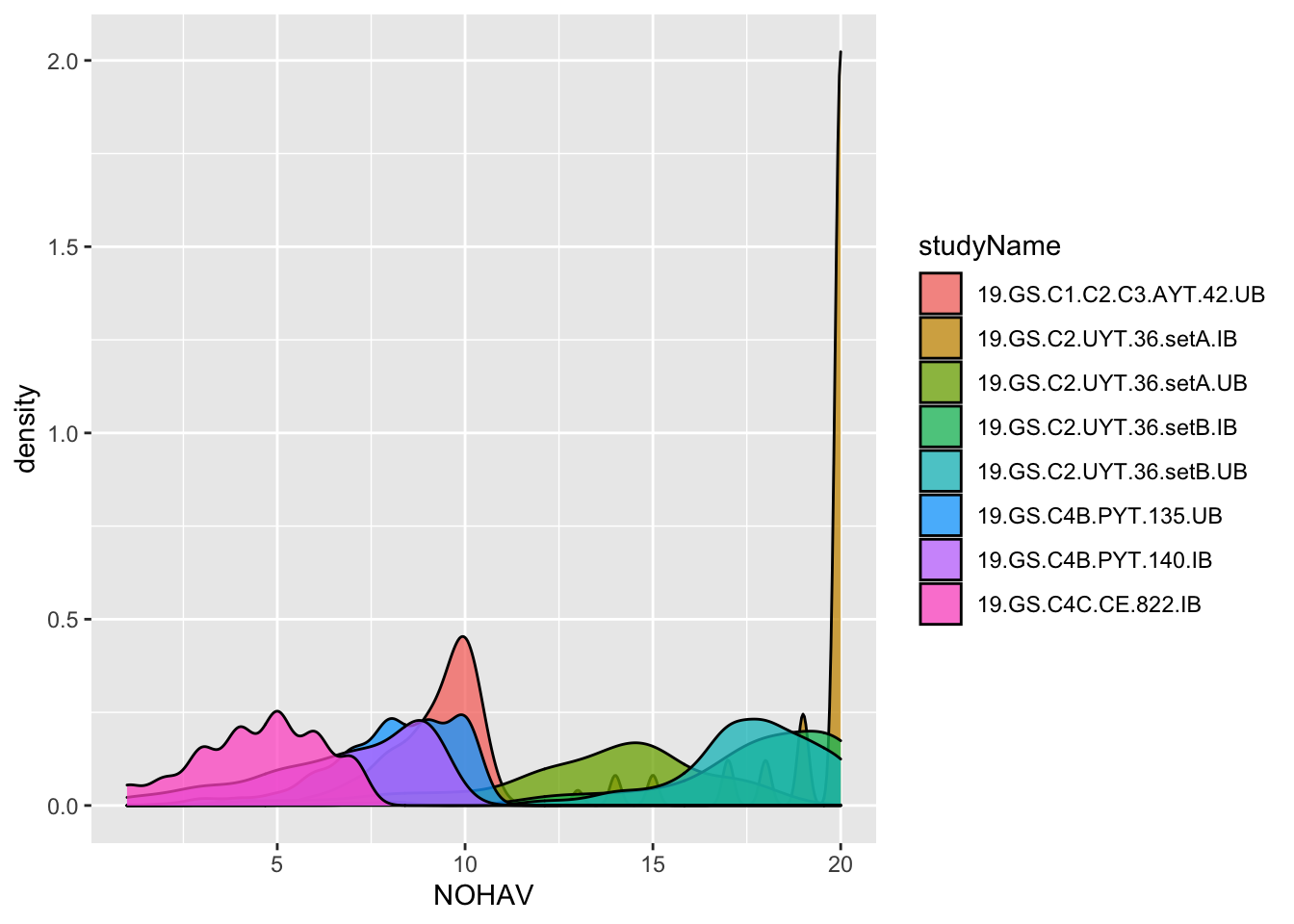
Maybe clearer to make a boxplot?
dbdata %>%
     # plot area in meters squared
     mutate(plotArea=plotWidth*plotLength) %>%
     ggplot(.,aes(x=plotArea,y=NOHAV, fill=studyName)) +
     geom_boxplot() + theme(axis.text.x = element_blank())
#> Warning: Removed 921 rows containing non-finite values
#> (stat_boxplot).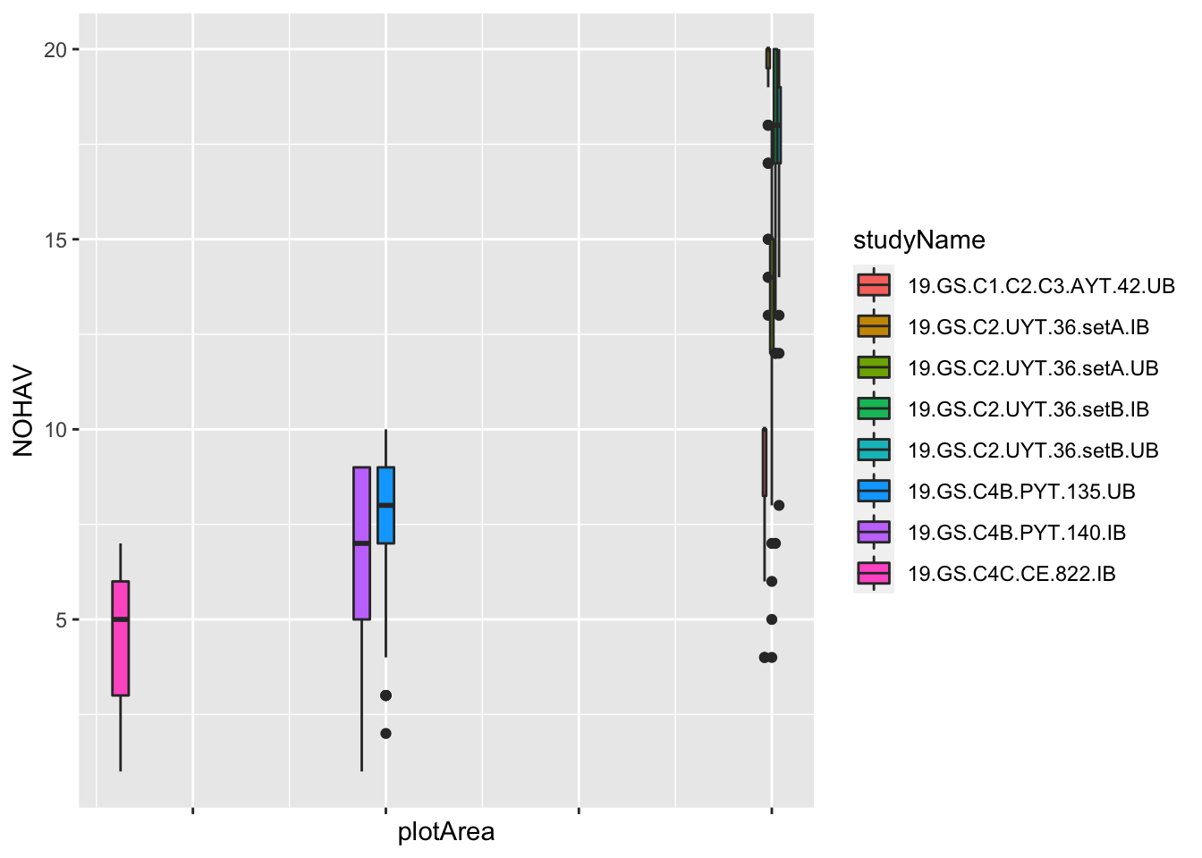
plantsPerPlot_choices<-dbdata %>%
     distinct(studyYear,studyName,plotWidth,plotLength,plantsPerPlot) %>%
     left_join(dbdata %>%
                    group_by(studyName) %>%
                    summarize(MaxNOHAV=max(NOHAV, na.rm=T))) %>%
          # plot area in meters squared
     mutate(plotArea=plotWidth*plotLength,
            # Number of plants per plot
            plantsPerPlot=MaxNOHAV,
            plantsPerPlot=ifelse(studyName=="19.GS.C2.UYT.36.setA.UB",20,plantsPerPlot)) %>%
     # exclude the empty genetic gain trial
     filter(studyName!="19geneticgainUB") %>%
     select(studyName,plotArea,MaxNOHAV,plantsPerPlot)
#> Warning in max(NOHAV, na.rm = T): no non-missing arguments
#> to max; returning -Inf
#> Joining, by = "studyName"
plantsPerPlot_choices %>% gt() #%>% tab_options(table.font.size = pct(67))| studyName | plotArea | MaxNOHAV | plantsPerPlot |
|---|---|---|---|
| 19.GS.C1.C2.C3.AYT.42.UB | 16.0 | 10 | 10 |
| 19.GS.C2.UYT.36.setA.IB | 16.0 | 20 | 20 |
| 19.GS.C2.UYT.36.setA.UB | 16.0 | 18 | 20 |
| 19.GS.C2.UYT.36.setB.IB | 16.0 | 20 | 20 |
| 19.GS.C2.UYT.36.setB.UB | 16.0 | 20 | 20 |
| 19.GS.C4B.PYT.135.UB | 8.0 | 10 | 10 |
| 19.GS.C4B.PYT.140.IB | 7.5 | 9 | 9 |
| 19.GS.C4C.CE.822.IB | 2.5 | 7 | 7 |
For the sake of this example, it is ‘ok’ to make choices on the basis I have just done.
As a data generator, in-house at each breeding program, no reason not to get the correct answer and repair the metadata on the database!
dbdata %<>%
     # remove the empty genetic gain trial
     filter(studyName!="19geneticgainUB") %>%
     select(-plantsPerPlot) %>%
     # join plantsPerPlot_choices to the trial data
     left_join(plantsPerPlot_choices) %>%
     # compute fresh root yield (FYLD) in tons per hectare
     mutate(PlantSpacing=plotArea/plantsPerPlot,
            FYLD=RTWT/(plantsPerPlot*PlantSpacing)*10)
#> Joining, by = "studyName"
dbdata %>% ggplot(.,aes(x=FYLD,fill=studyName)) + geom_density(alpha=0.75)
#> Warning: Removed 133 rows containing non-finite values
#> (stat_density).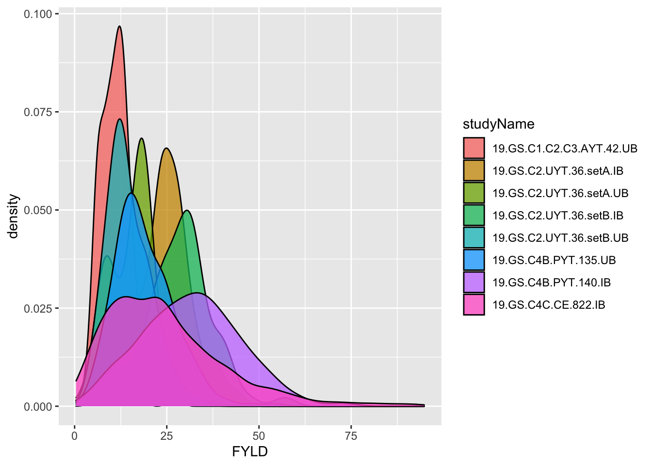
Additional things to compute:
- log-transform yield traits: this is a habit based on experience. Linear mixed-models should have normally distributed homoskedastic residuals, if they don’t log-transform the response variable often helps. For FYLD and related traits, I always log-transform.
# I log transform yield traits
# to satisfy homoskedastic residuals assumption
# of linear mixed models
dbdata %<>%
     mutate(DYLD=FYLD*(DM/100),
            logFYLD=log(FYLD),
            logDYLD=log(DYLD),
            PropNOHAV=NOHAV/plantsPerPlot)
# remove non transformed / per-plot (instead of per area) traits
dbdata %<>% select(-RTWT,-FYLD,-DYLD)
dbdata %>% ggplot(.,aes(x=logFYLD,fill=studyName)) + geom_density(alpha=0.75)
#> Warning: Removed 133 rows containing non-finite values
#> (stat_density).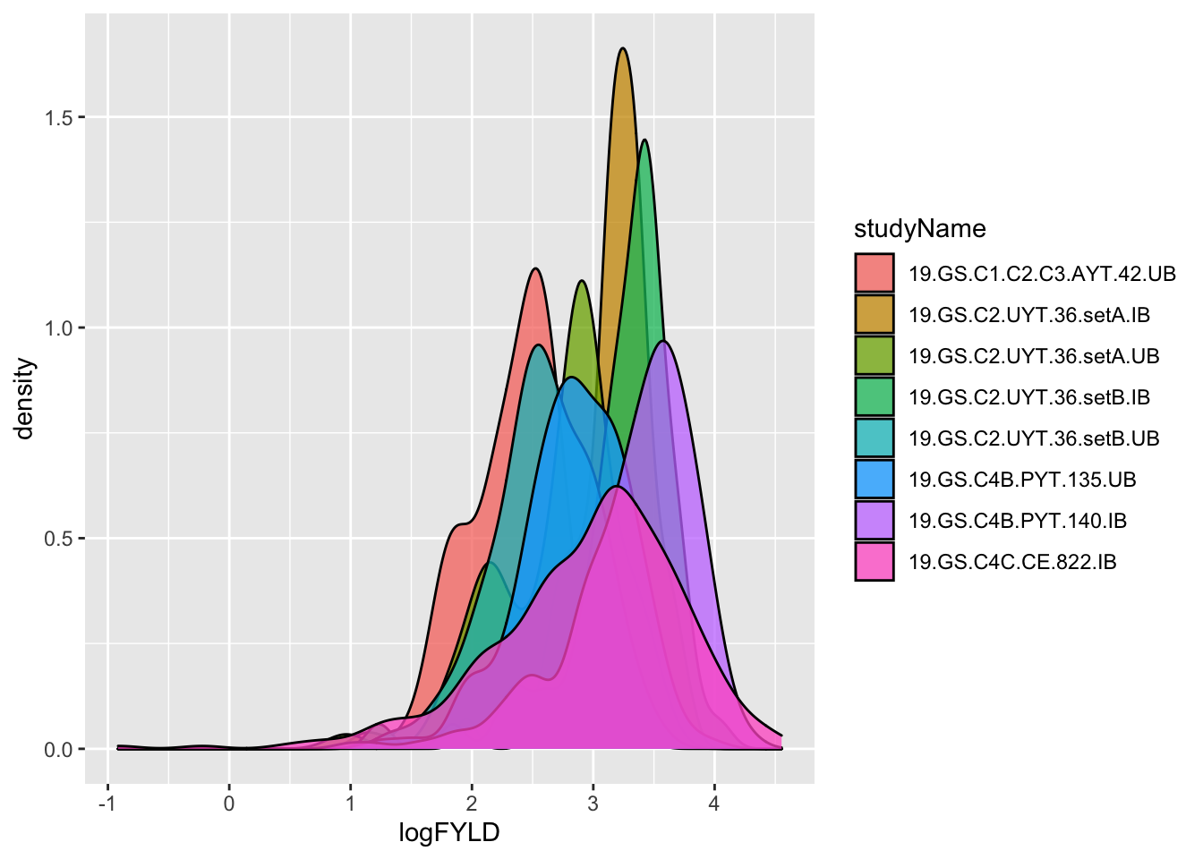
Debatable whether this is better. Let’s not dwell on it. Onward!
SUGGESTION: For individuals working this manual, consider making different, or no transformations as you see fit, with your own data. Even better, set-up a direct comparison of results with- vs. without-transformation.*