15 Predict crosses
Context and Purpose:
Upstream: Section @ref() -
Downstream:
Inputs:
Expected outputs:
We are finally (almost) ready to predict the performance of potential crosses. We have a few inputs to set-up.
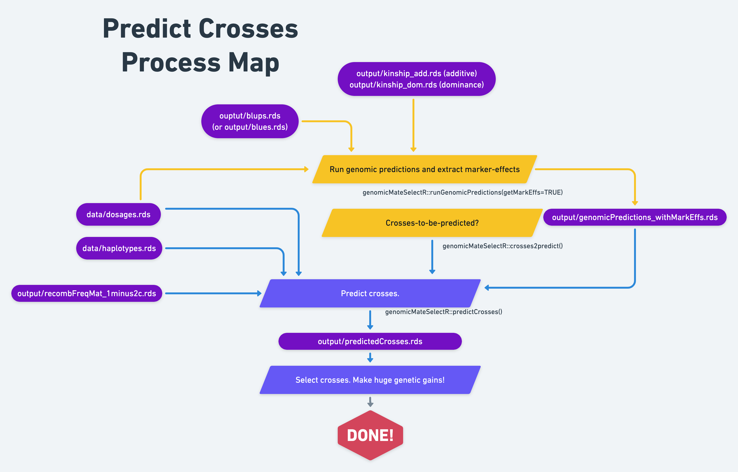
15.2 Load inputs and set-up
Much the same as in the section on parent-wise cross-validation.
# GENOMIC RELATIONSHIP MATRIX
grms<-list(A=readRDS(file=here::here("output","kinship_add.rds")))

# BLUPs
blups<-readRDS(here::here("output","blups.rds")) %>%
     # based on cross-validation, decided to exclude MCMDS from this analysis
     filter(Trait != "MCMDS") %>%
     # need to rename the "blups" list to comply with the runCrossVal function
     rename(TrainingData=blups) %>%
     dplyr::select(Trait,TrainingData) %>%
     # need also to remove phenotyped-but-not-genotyped lines
     mutate(TrainingData=map(TrainingData,
                             ~filter(.,germplasmName %in% rownames(grms$A)) %>%
                                  # rename the germplasmName column to GID
                                  rename(GID=germplasmName)))

# DOSAGE MATRIX
## Dosages are also needed for runGenomicPredictions() when getMarkEffs=TRUE
## Reason is that they are used to extra SNP effects from GBLUP models
dosages<-readRDS(here::here("data","dosages.rds"))

# SELECTION INDEX
SIwts<-c(DM=15,
         logFYLD=20,
         logDYLD=20)
15.3 Get marker effects
First, in the chapter where we predicted GEBV, we used the runGenomicPredictions() function, which implements a GBLUP model, to predict GEBV.
We need to re-run runGenomicPredictions(), this time using the getMarkEffs=TRUE option, this will “backsolve” the RR-BLUP marker effect solutions from the GBLUP solutions, using the backsolveSNPeff() function under-the-hood.
Refer to the runGenomicPredictions() documentation here and this section of the vignette for more details.
The output SNP-effects will be formatted ready to be input into the predictCrosses() function.
gpreds_withMarkEffs<-runGenomicPredictions(modelType = "A",
                                           selInd = T, SIwts = SIwts,
                                           getMarkEffs = TRUE,
                                           dosages = dosages,
                                           blups = blups,
                                           grms = grms,
                                           ncores=3)
Save the results
Notice that there is now a additional list-type column with the label “allelesubsnpeff” indicating that, because we ran an additive-only model, these SNP-effects represent predictions of allele substitution effects.
gpreds_withMarkEffs$genomicPredOut[[1]]
#> # A tibble: 3 × 5
#>   Trait   gblups       varcomps   fixeffs    allelesubsnpeff
#>   <chr>   <list>       <list>     <list>     <list>
#> 1 DM      <tibble [96… <df [2 × … <df [1 × … <dbl [3,986 × …
#> 2 logFYLD <tibble [96… <df [2 × … <df [1 × … <dbl [3,986 × …
#> 3 logDYLD <tibble [96… <df [2 × … <df [1 × … <dbl [3,986 × …
Just to show, they are a single column matrix with rownames labelling each marker.
gpreds_withMarkEffs$genomicPredOut[[1]]$allelesubsnpeff[[1]][1:5,]
#>  1_652699_G_C  1_868970_G_T  1_943129_T_A 1_1132830_A_T
#> -0.0019610837 -0.0016106918 -0.0008841766 -0.0017600501
#> 1_1310706_A_T
#> -0.0012963110
15.4 Crosses-to-predict
The predictCrosses() function will also need a data.frame indicating what pairs of parents we want to predict crosses for.
As a convenience, we can use the crosses2predict() function to make such a data.frame from a vector of genotype ID’s.
A realistic approach, is to choose a set of parents based on their GEBV, but more than we’d actually like to actually make crosses with.
It is still somewhat computationally intensive to predict the variances and covariances of traits for each cross, so we can’t quite predict all possible pairwise crosses… definitely not on our laptops for this example.
Here, as an example, picking the top 10 candidate parents:
# Access the predicted GEBV
top10parents<-gpreds_withMarkEffs$gblups[[1]] %>%
     # Arrange in descending order based on the SELIND
     arrange(desc(SELIND)) %>%
     # I'll pick the top 10 parents
     slice(1:10) %$%
     # And extract their GID to a vector
     GID
CrossesToPredict<-crosses2predict(top10parents)
CrossesToPredict %>% head
#> # A tibble: 6 × 2
#>   sireID          damID
#>   <chr>           <chr>
#> 1 TMS13F1307P0008 TMS13F1307P0008
#> 2 TMS13F1307P0008 TMS14F1035P0004
#> 3 TMS13F1307P0008 TMS14F1262P0002
#> 4 TMS13F1307P0008 TMS19F1091P0065
#> 5 TMS13F1307P0008 TMS14F1303P0012
#> 6 TMS13F1307P0008 TMS14F1312P0003So we have 55 crosses of the top 10 parents to make predictions for.
15.5 Run predictCrosses()
Additional inputs we will need: “haplotype matrix” and “recombination frequency matrix.”
# HAPLOTYPE MATRIX
## keep only haplos for candidate parents we want to predict crosses for
## those which will be used in prediction, saves memory
haploMat<-readRDS(file=here::here("data","haplotypes.rds"))
parenthaps<-sort(c(paste0(top10parents,"_HapA"),
                   paste0(top10parents,"_HapB")))
haploMat<-haploMat[parenthaps,]

# RECOMBINATION FREQUENCY MATRIX
recombFreqMat<-readRDS(file=here::here("output","recombFreqMat_1minus2c.rds"))
Let’s go!
starttime<-proc.time()[3]
crossPreds<-predictCrosses(modelType="A",
                           selInd = T, SIwts = SIwts,
                           CrossesToPredict=CrossesToPredict,
                           snpeffs=gpreds_withMarkEffs$genomicPredOut[[1]],
                           haploMat=haploMat,
                           dosages = dosages[top10parents,],
                           recombFreqMat=recombFreqMat,
                           ncores=10)
elapsed<-proc.time()[3]-starttime; elapsed/6015.6 Select crosses to make
crossPreds
#> # A tibble: 1 × 2
#>   tidyPreds          rawPreds
#>   <list>             <list>
#> 1 <tibble [220 × 9]> <named list [2]>
Output of predictCrosses() is a tibble. Two columns, 1 row. Column 1 (tidyPreds) has cleaned-up “tidy” predictions. Column 2 (rawPreds) has more detailed output.
crossPreds$tidyPreds[[1]] %>% str
#> tibble [220 × 9] (S3: tbl_df/tbl/data.frame)
#>  $ sireID        : chr [1:220] "TMS13F1307P0008" "TMS13F1307P0008" "TMS13F1307P0008" "TMS13F1307P0008" ...
#>  $ damID         : chr [1:220] "TMS13F1307P0008" "TMS13F1307P0008" "TMS13F1307P0008" "TMS13F1307P0008" ...
#>  $ Nsegsnps      : int [1:220] 1281 1281 1281 1281 2048 2048 2048 2048 1762 1762 ...
#>  $ predOf        : chr [1:220] "BV" "BV" "BV" "BV" ...
#>  $ Trait         : chr [1:220] "SELIND" "DM" "logFYLD" "logDYLD" ...
#>  $ predMean      : num [1:220] 16.48943 1.04623 -0.00208 0.04188 16.39717 ...
#>  $ predVar       : num [1:220] 6.732467 0.025773 0.000276 0.000279 8.111941 ...
#>  $ predSD        : num [1:220] 2.5947 0.1605 0.0166 0.0167 2.8481 ...
#>  $ predUsefulness: num [1:220] 23.4173 1.4749 0.0423 0.0864 24.0017 ...
Remember that the “usefulness” (predUsefulness) here, or UC for short, is equal to a prediction of the expected mean of the top fraction of progeny from each cross \(\hat{UC} = \hat{\mu} + i \times \hat{\sigma}\). This is also called the “superior progeny mean” in the literature. Actually, the user has the option to modify the expected, standardized selection intensity (\(\boldsymbol{i}\)) either in advance with the stdSelInt= argument to predictCrosses() or after-the-fact; the default is a value of 2.67, corresponding to selecting the top 1% of offspring for the cross you will be making.
So let’s say you want to make only the top 10 of the 55 predicted crosses:
top10crosses<-crossPreds$tidyPreds[[1]] %>%
     filter(Trait=="SELIND") %>%
     dplyr::select(-predVar) %>%
     arrange(desc(predUsefulness)) %>%
     slice(1:10)
top10crosses
#> # A tibble: 10 × 8
#>    sireID     damID    Nsegsnps predOf Trait predMean predSD
#>    <chr>      <chr>       <int> <chr>  <chr>    <dbl>  <dbl>
#>  1 TMS14F103… TMS14F1…     1429 BV     SELI…     16.3   3.08
#>  2 TMS13F130… TMS14F1…     2048 BV     SELI…     16.4   2.85
#>  3 TMS13F130… TMS13F1…     1281 BV     SELI…     16.5   2.59
#>  4 TMS14F103… TMS14F1…     2099 BV     SELI…     15.2   2.87
#>  5 TMS13F130… TMS14F1…     1762 BV     SELI…     15.3   2.62
#>  6 TMS14F103… TMS19F1…     2013 BV     SELI…     14.3   2.86
#>  7 TMS14F103… TMS14F1…     2260 BV     SELI…     14.2   2.83
#>  8 TMS13F130… TMS19F1…     1934 BV     SELI…     14.4   2.60
#>  9 TMS13F130… TMS14F1…     2136 BV     SELI…     14.3   2.57
#> 10 TMS14F126… TMS14F1…     1118 BV     SELI…     14.1   2.65
#> # … with 1 more variable: predUsefulness <dbl>
And thus we have a crossing plan! Congratulations!
15.7 Non-additive effects models
Links to information on these models are provided in the previous section introducing genomic mate selection.
The vignette in genomicMateSelectR entitled “Genomic prediction with non-additive effects”provides a complete tutorial on how to execute these models and predicting cross-performance with them.