Results
2021-July-26
Last updated: 2021-08-04
Checks: 7 0
Knit directory: implementGMSinCassava/
This reproducible R Markdown analysis was created with workflowr (version 1.6.2). The Checks tab describes the reproducibility checks that were applied when the results were created. The Past versions tab lists the development history.
Great! Since the R Markdown file has been committed to the Git repository, you know the exact version of the code that produced these results.
Great job! The global environment was empty. Objects defined in the global environment can affect the analysis in your R Markdown file in unknown ways. For reproduciblity it’s best to always run the code in an empty environment.
The command set.seed(20210504) was run prior to running the code in the R Markdown file. Setting a seed ensures that any results that rely on randomness, e.g. subsampling or permutations, are reproducible.
Great job! Recording the operating system, R version, and package versions is critical for reproducibility.
Nice! There were no cached chunks for this analysis, so you can be confident that you successfully produced the results during this run.
Great job! Using relative paths to the files within your workflowr project makes it easier to run your code on other machines.
Great! You are using Git for version control. Tracking code development and connecting the code version to the results is critical for reproducibility.
The results in this page were generated with repository version f6f58f0. See the Past versions tab to see a history of the changes made to the R Markdown and HTML files.
Note that you need to be careful to ensure that all relevant files for the analysis have been committed to Git prior to generating the results (you can use wflow_publish or wflow_git_commit). workflowr only checks the R Markdown file, but you know if there are other scripts or data files that it depends on. Below is the status of the Git repository when the results were generated:
Ignored files:
    Ignored:    .DS_Store
    Ignored:    .Rhistory
    Ignored:    .Rproj.user/
    Ignored:    analysis/.DS_Store
    Ignored:    code/.DS_Store
    Ignored:    data/.DS_Store

Untracked files:
    Untracked:  analysis/speedUpPredCrossVar.Rmd
    Untracked:  data/AllChrom_RefPanelAndGSprogeny_ReadyForGP_72719.bed
    Untracked:  data/AllChrom_RefPanelAndGSprogeny_ReadyForGP_72719.bim
    Untracked:  data/AllChrom_RefPanelAndGSprogeny_ReadyForGP_72719.fam
    Untracked:  data/AllChrom_RefPanelAndGSprogeny_ReadyForGP_72719.hap.gz
    Untracked:  data/AllChrom_RefPanelAndGSprogeny_ReadyForGP_72719.log
    Untracked:  data/AllChrom_RefPanelAndGSprogeny_ReadyForGP_72719.nosex
    Untracked:  data/AllChrom_RefPanelAndGSprogeny_ReadyForGP_72719.sample
    Untracked:  data/AllChrom_RefPanelAndGSprogeny_ReadyForGP_72719.vcf.gz
    Untracked:  data/DatabaseDownload_2021May04/
    Untracked:  data/blups_forCrossVal.rds
    Untracked:  data/config.txt
    Untracked:  data/config_mw.txt
    Untracked:  data/dosages_IITA_2021May13.rds
    Untracked:  data/dosages_IITA_filtered_2021May13.rds
    Untracked:  data/genmap_2021Aug02.rds
    Untracked:  data/genmap_2021May13.rds
    Untracked:  data/haps_IITA_2021May13.rds
    Untracked:  data/haps_IITA_filtered_2021May13.rds
    Untracked:  data/recombFreqMat_1minus2c_2021May13.rds
    Untracked:  output/Cassava_HMII_V3_Marning_imputation_6-18-21.samples
    Untracked:  output/IITA_CleanedTrialData_2021May10.rds
    Untracked:  output/IITA_ExptDesignsDetected_2021May10.rds
    Untracked:  output/IITA_blupsForModelTraining_twostage_asreml_2021May10.rds
    Untracked:  output/IITA_trials_NOT_identifiable.csv
    Untracked:  output/alphaAssignOutput_iita_pedigree.txt.dams
    Untracked:  output/alphaAssignOutput_iita_pedigree.txt.dams.full
    Untracked:  output/alphaAssignOutput_iita_pedigree.txt.pedigree
    Untracked:  output/alphaAssignOutput_iita_pedigree.txt.pedigree.top
    Untracked:  output/alphaAssignOutput_iita_pedigree.txt.sires
    Untracked:  output/alphaAssignOutput_iita_pedigree.txt.sires.full
    Untracked:  output/crossValPredsA.rds
    Untracked:  output/crossValPredsAD.rds
    Untracked:  output/cvAD_1rep_markerEffects.rds
    Untracked:  output/cvAD_1rep_meanPredAccuracy.rds
    Untracked:  output/cvAD_1rep_parentfolds.rds
    Untracked:  output/cvAD_1rep_predAccuracy.rds
    Untracked:  output/cvAD_1rep_predMeans.rds
    Untracked:  output/cvAD_1rep_predVars.rds
    Untracked:  output/cvAD_1rep_varPredAccuracy.rds
    Untracked:  output/cvAD_5rep5fold_markerEffects.rds
    Untracked:  output/cvAD_5rep5fold_meanPredAccuracy.rds
    Untracked:  output/cvAD_5rep5fold_parentfolds.rds
    Untracked:  output/cvAD_5rep5fold_predMeans.rds
    Untracked:  output/cvAD_5rep5fold_predVars.rds
    Untracked:  output/cvAD_5rep5fold_varPredAccuracy.rds
    Untracked:  output/cvDirDom_1Mb_50kb_pt5_predAccuracy.rds
    Untracked:  output/cvDirDom_1Mb_50kb_pt6_predAccuracy.rds
    Untracked:  output/cvDirDom_1Mb_50kb_pt8_predAccuracy.rds
    Untracked:  output/cvDirDom_1Mb_50kb_pt9_predAccuracy.rds
    Untracked:  output/cvDirDom_5rep5fold_markerEffects.rds
    Untracked:  output/cvDirDom_5rep5fold_meanPredAccuracy.rds
    Untracked:  output/cvDirDom_5rep5fold_parentfolds.rds
    Untracked:  output/cvDirDom_5rep5fold_predMeans.rds
    Untracked:  output/cvDirDom_5rep5fold_predVars.rds
    Untracked:  output/cvDirDom_5rep5fold_varPredAccuracy.rds
    Untracked:  output/cvMeanPredAccuracyA.rds
    Untracked:  output/cvMeanPredAccuracyAD.rds
    Untracked:  output/cvPredMeansA.rds
    Untracked:  output/cvPredMeansAD.rds
    Untracked:  output/cvVarPredAccuracyA.rds
    Untracked:  output/cvVarPredAccuracyAD.rds
    Untracked:  output/genomicMatePredictions_top121parents_ModelAD.csv
    Untracked:  output/genomicMatePredictions_top121parents_ModelAD.rds
    Untracked:  output/genomicMatePredictions_top121parents_ModelDirDom.csv
    Untracked:  output/genomicMatePredictions_top121parents_ModelDirDom.rds
    Untracked:  output/genomicPredictions_ModelAD.csv
    Untracked:  output/genomicPredictions_ModelAD.rds
    Untracked:  output/genomicPredictions_ModelDirDom.csv
    Untracked:  output/genomicPredictions_ModelDirDom.rds
    Untracked:  output/kinship_A_IITA_2021May13.rds
    Untracked:  output/kinship_D_IITA_2021May13.rds
    Untracked:  output/kinship_domGenotypic_IITA_2021July5.rds
    Untracked:  output/markEffsTest.rds
    Untracked:  output/markerEffects.rds
    Untracked:  output/markerEffectsA.rds
    Untracked:  output/markerEffectsAD.rds
    Untracked:  output/maxNOHAV_byStudy.csv
    Untracked:  output/obsCrossMeansAndVars.rds
    Untracked:  output/parentfolds.rds
    Untracked:  output/ped2check_genome.rds
    Untracked:  output/ped2genos.txt
    Untracked:  output/pednames2keep.txt
    Untracked:  output/pednames_Prune100_25_pt25.log
    Untracked:  output/pednames_Prune100_25_pt25.nosex
    Untracked:  output/pednames_Prune100_25_pt25.prune.in
    Untracked:  output/pednames_Prune100_25_pt25.prune.out
    Untracked:  output/potential_dams.txt
    Untracked:  output/potential_sires.txt
    Untracked:  output/predVarTest.rds
    Untracked:  output/samples2keep_IITA_2021May13.txt
    Untracked:  output/samples2keep_IITA_MAFpt01_prune50_25_pt98.log
    Untracked:  output/samples2keep_IITA_MAFpt01_prune50_25_pt98.nosex
    Untracked:  output/samples2keep_IITA_MAFpt01_prune50_25_pt98.prune.in
    Untracked:  output/samples2keep_IITA_MAFpt01_prune50_25_pt98.prune.out
    Untracked:  output/samples2keep_notInPHGdb.txt
    Untracked:  output/stdcvDirDom_1Mb_50kb_pt5_predAccuracy.rds
    Untracked:  output/stdcvDirDom_1Mb_50kb_pt6_predAccuracy.rds
    Untracked:  output/stdcvDirDom_1Mb_50kb_pt8_predAccuracy.rds
    Untracked:  output/stdcvDirDom_1Mb_50kb_pt9_predAccuracy.rds
    Untracked:  output/stdcv_AD_predAccuracy.rds
    Untracked:  output/stdcv_DirDom_predAccuracy.rds
    Untracked:  output/test_cvAD_markerEffects.rds
    Untracked:  output/test_cvAD_meanPredAccuracy.rds
    Untracked:  output/test_cvAD_parentfolds.rds
    Untracked:  output/test_cvAD_predAccuracy.rds
    Untracked:  output/test_cvAD_predMeans.rds
    Untracked:  output/test_cvAD_predVars.rds
    Untracked:  output/test_cvAD_varPredAccuracy.rds
    Untracked:  output/top50crosses.csv
    Untracked:  output/verified_ped.txt
Note that any generated files, e.g. HTML, png, CSS, etc., are not included in this status report because it is ok for generated content to have uncommitted changes.
These are the previous versions of the repository in which changes were made to the R Markdown (analysis/07-Results.Rmd) and HTML (docs/07-Results.html) files. If you’ve configured a remote Git repository (see ?wflow_git_remote), click on the hyperlinks in the table below to view the files as they were in that past version.
| File | Version | Author | Date | Message |
|---|---|---|---|---|
| Rmd | af71a07 | wolfemd | 2021-08-04 | Add optimize marker density for speed results examination and recommendations. |
| html | ba8527c | wolfemd | 2021-08-02 | Build site. |
| Rmd | 5e7bc99 | wolfemd | 2021-08-02 | Results now include both “standard” and parent-wise cross-validation accuracies and plots of cross mean/variance predictions. Ready to knit and publish + push to FTP. |
| html | 769fe81 | wolfemd | 2021-07-29 | Build site. |
| Rmd | bc85a7d | wolfemd | 2021-07-29 | Polished and ready to go. |
| html | baa7d80 | wolfemd | 2021-07-29 | Build site. |
| Rmd | 5a53779 | wolfemd | 2021-07-29 | Publish the nearly complete and polished version of the project. |
| html | 934141c | wolfemd | 2021-07-14 | Build site. |
| html | cc1eb4b | wolfemd | 2021-07-14 | Build site. |
| Rmd | 772750a | wolfemd | 2021-07-14 | DirDom model and selection index calc fully integrated functions. |
The summaries below correspond to the results of analyses outlined here and linked in the navbar above.
- Preliminary summaries of the population, the data, results of pedigree validation,
- Prediction accuracy estimates
- Genomic Predictions and Genomic mate selection.
- Optimize marker density for speed: Test whether marker density can be reduced to save compute time (enabling us to predict more crosses) without sacrificing prediction accuracy. Use both standard and parent-wise cross-validation and LD-based pruning of markers.
Preliminary summaries
Raw data
Summary of the number of unique plots, locations, years, etc. in the cleaned plot-basis data (output/IITA_ExptDesignsDetected_2021May10.rds, download from FTP). See the data cleaning step here for details.
library(tidyverse); library(magrittr); library(ragg)
rawdata<-readRDS(file=here::here("output","IITA_ExptDesignsDetected_2021May10.rds"))
rawdata %>%
  summarise(Nplots=nrow(.),
            across(c(locationName,studyYear,studyName,TrialType,GID), ~length(unique(.)),.names = "N_{.col}")) %>%
  rmarkdown::paged_table()
This is not the same number of clones as are expected to be genotyped-and-phenotyped.
Next, a break down of the plots based on the trial design and TrialType (really a grouping of the population that is breeding program specific), captured by two logical variables, CompleteBlocks and IncompleteBlocks.
rawdata %>%
  count(TrialType,CompleteBlocks,IncompleteBlocks) %>%
  spread(TrialType,n) %>%
  rmarkdown::paged_table()
Next, look at breakdown of plots by TrialType (rows) and locations (columns):
rawdata %>%
  count(locationName,TrialType) %>%
  spread(locationName,n) %>%
rmarkdown::paged_table()traits<-c("MCMDS","DM","PLTHT","BRNHT1","BRLVLS","HI",
"logDYLD", # <-- logDYLD now included.
"logFYLD","logTOPYLD","logRTNO","TCHART","LCHROMO","ACHROMO","BCHROMO")
rawdata %>%
select(locationName,studyYear,studyName,TrialType,any_of(traits)) %>%
pivot_longer(cols = any_of(traits), values_to = "Value", names_to = "Trait") %>%
ggplot(.,aes(x=Value,fill=Trait)) + geom_histogram() + facet_wrap(~Trait, scales='free') +
theme_bw() + scale_fill_viridis_d() +
labs(title = "Distribution of Raw Phenotypic Values")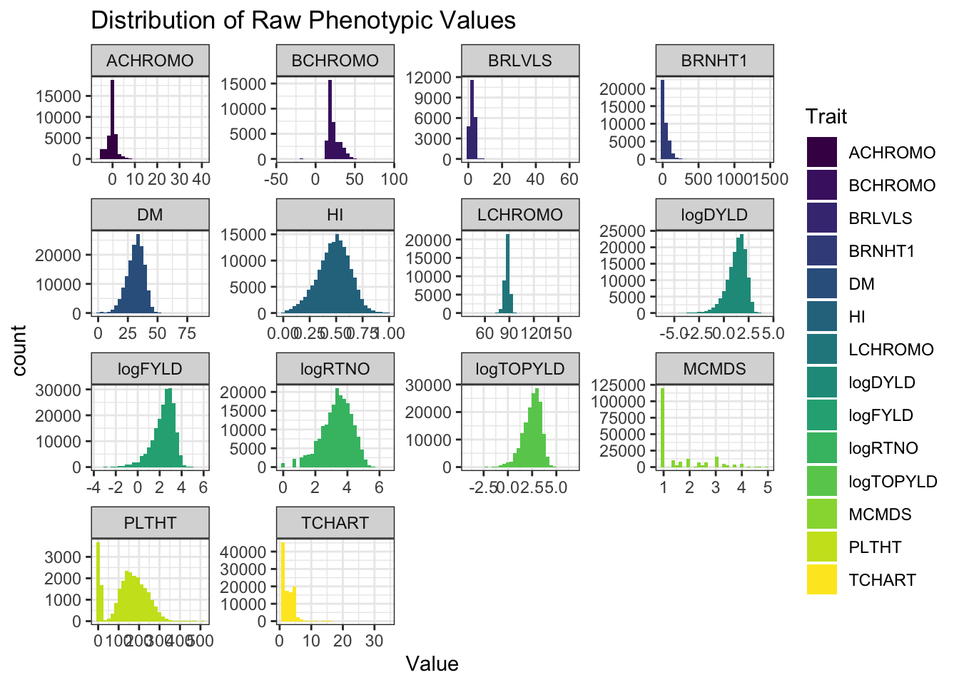
| Version | Author | Date |
|---|---|---|
| cc1eb4b | wolfemd | 2021-07-14 |
How many genotyped-and-phenotyped clones?
genotypedAndPhenotypedClones<-rawdata %>%
  select(locationName,studyYear,studyName,TrialType,germplasmName,FullSampleName,GID,any_of(traits)) %>%
  pivot_longer(cols = any_of(traits), values_to = "Value", names_to = "Trait") %>%
  filter(!is.na(Value),!is.na(FullSampleName)) %>%
  distinct(germplasmName,FullSampleName,GID)
There are 8149 genotyped-and-phenotyped clones!
genotypedAndPhenotypedClones %>%
  rmarkdown::paged_table()
BLUPs
Summarize the BLUPs from the training data, leveraging for each clone data across trials/locations without genomic information and to be used as input for genomic prediction downstream (data/blups_forCrossVal.rds, download from FTP). See the mixed-model analysis step here and a subsequent processing step here for details.
blups<-readRDS(file=here::here("data","blups_forCrossVal.rds"))
gidWithBLUPs<-blups %>% select(Trait,blups) %>% unnest(blups) %$% unique(GID)
rawdata %>%
  select(observationUnitDbId,GID,any_of(blups$Trait)) %>%
  pivot_longer(cols = any_of(blups$Trait),
               names_to = "Trait",
               values_to = "Value",values_drop_na = T) %>%
  filter(GID %in% gidWithBLUPs) %>%
  group_by(Trait) %>%
  summarize(Nplots=n()) %>%
  ungroup() %>%
  left_join(blups %>%
              mutate(Nclones=map_dbl(blups,~nrow(.)),
                     avgREL=map_dbl(blups,~mean(.$REL)),
                     Vg=map_dbl(varcomp,~.["GID!GID.var","component"]),
                     Ve=map_dbl(varcomp,~.["R!variance","component"]),
                     H2=Vg/(Vg+Ve)) %>%
              select(-blups,-varcomp)) %>%
  mutate(across(is.numeric,~round(.,3))) %>% arrange(desc(H2)) %>%
rmarkdown::paged_table()Nplots,Nclones: the number of unique plots and clones per traitavgREL: the mean reliability of BLUPs, where for the jth clone, \(REL_j = 1 - \frac{PEV_j}{V_g}\)Vg,Ve,H2: the genetic and residual variance components and the broad sense heritability (\(H^2=\frac{V_g}{V_g+V_e}\)).
blups %>%
  select(Trait,blups) %>%
  unnest(blups) %>%
  ggplot(.,aes(x=drgBLUP,fill=Trait)) + geom_histogram() + facet_wrap(~Trait, scales='free') +
  theme_bw() + scale_fill_viridis_d() + theme(legend.position = 'none') +
  labs(title = "Distribution of de-regressed BLUP Values")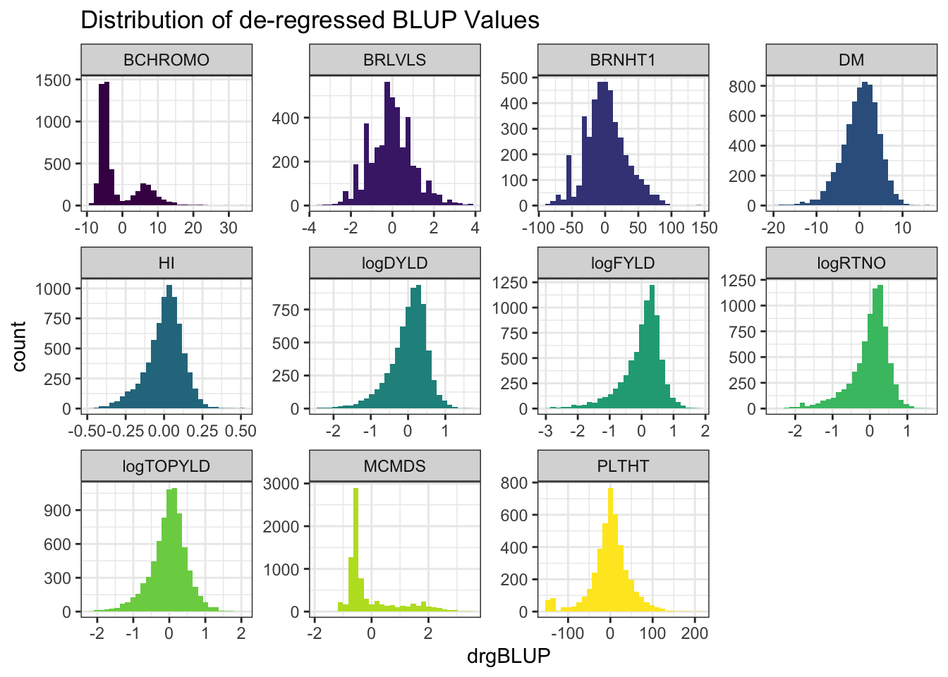
- de-regressed BLUPs or \(drgBLUP_j = \frac{BLUP_j}{REL_j}\)
blups %>%
  select(Trait,blups) %>%
  unnest(blups) %>%
  ggplot(.,aes(x=Trait,y=REL,fill=Trait)) + geom_boxplot(notch=T) + #facet_wrap(~Trait, scales='free') +
  theme_bw() + scale_fill_viridis_d() +
  theme(axis.text.x = element_text(angle=90),
        legend.position = 'none') +
  labs(title = "Distribution of BLUP Reliabilities")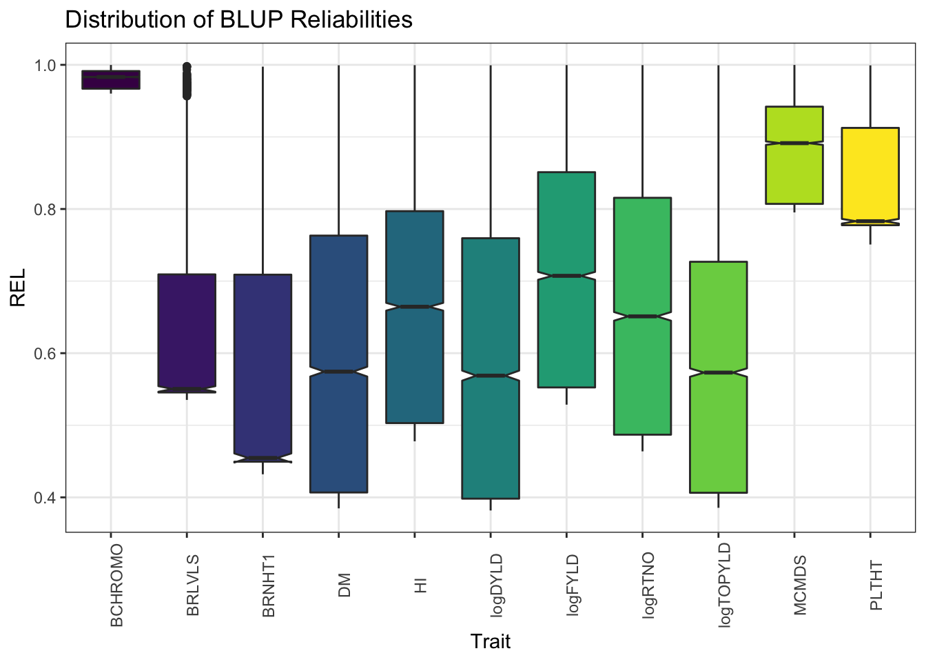
Marker density and distribution
Summarize the marker data (data/dosages_IITA_filtered_2021May13.rds, download from FTP). See the pre-processing steps here.
library(tidyverse); library(magrittr);
getwd()
[1] "/Users/mw489/Google Drive/NextGenGS/implementGMSinCassava"snps<-readRDS(file=here::here("data","dosages_IITA_filtered_2021May13.rds"))
mrks<-colnames(snps) %>%
tibble(SNP_ID=.) %>%
separate(SNP_ID,c("Chr","Pos","Allele"),"_") %>%
mutate(Chr=as.integer(gsub("S","",Chr)),
Pos=as.numeric(Pos))
rm(snps);
mrks %>%
ggplot(.,aes(x=Pos,fill=as.character(Chr))) + geom_histogram() +
facet_wrap(~Chr,scales = 'free') + theme_bw() +
scale_fill_viridis_d() + theme(legend.position = 'none',
axis.text.x = element_text(angle=90))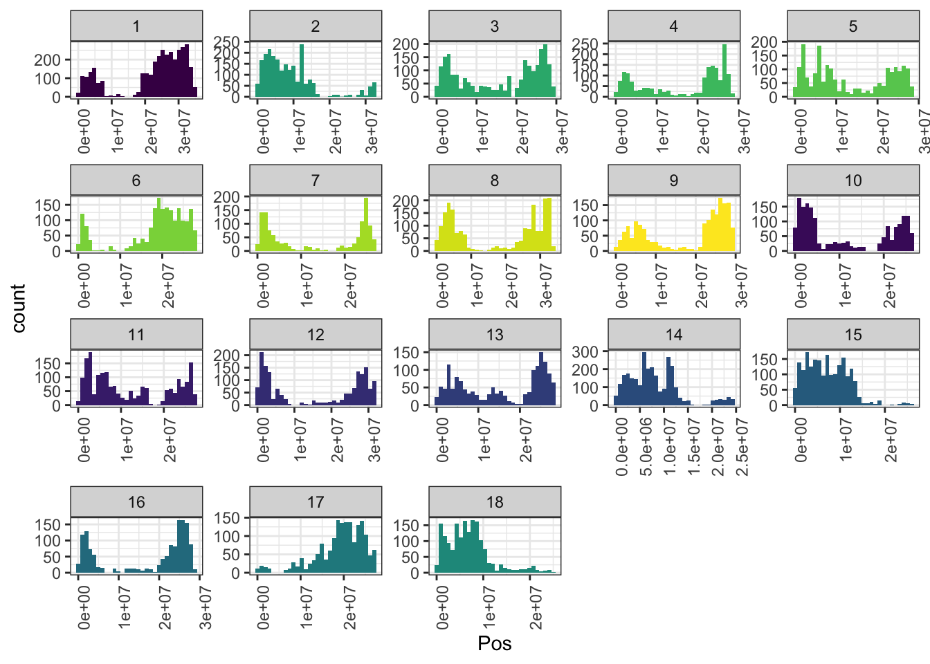
| Version | Author | Date |
|---|---|---|
| baa7d80 | wolfemd | 2021-07-29 |
In total, 34981 SNPs genome-wide. Broken down by chromosome:
mrks %>% count(Chr,name = "Nsnps") %>% rmarkdown::paged_table()Pedigree validation
Introduced new downstream procedures (the parent-wise cross-validation, which rely on a trusted pedigree. To support this, introduced a new pedigree-validation step. The pedigree and validation results are summarized below.
The verified pedigree (output/verified_ped.txt), can be downloaded from the FTP here).
library(tidyverse); library(magrittr);
ped2check_genome<-readRDS(file=here::here("output","ped2check_genome.rds"))
ped2check_genome %<>%
  select(IID1,IID2,Z0,Z1,Z2,PI_HAT)
ped2check<-read.table(file=here::here("output","ped2genos.txt"),
                      header = F, stringsAsFactors = F) %>%
  rename(FullSampleName=V1,DamID=V2,SireID=V3)
ped2check %<>%
  select(FullSampleName,DamID,SireID) %>%
  inner_join(ped2check_genome %>%
               rename(FullSampleName=IID1,DamID=IID2) %>%
               bind_rows(ped2check_genome %>%
                           rename(FullSampleName=IID2,DamID=IID1))) %>%
  distinct %>%
  mutate(FemaleParent=case_when(Z0<0.32 & Z1>0.67~"Confirm",
                                       SireID==DamID & PI_HAT>0.6 & Z0<0.3 & Z2>0.32~"Confirm",
                                       TRUE~"Reject")) %>%
  select(-Z0,-Z1,-Z2,-PI_HAT) %>%
  inner_join(ped2check_genome %>%
               rename(FullSampleName=IID1,SireID=IID2) %>%
               bind_rows(ped2check_genome %>%
                           rename(FullSampleName=IID2,SireID=IID1))) %>%
  distinct %>%
  mutate(MaleParent=case_when(Z0<0.32 & Z1>0.67~"Confirm",
                                       SireID==DamID & PI_HAT>0.6 & Z0<0.3 & Z2>0.32~"Confirm",
                                       TRUE~"Reject")) %>%
  select(-Z0,-Z1,-Z2,-PI_HAT)
rm(ped2check_genome)

ped2check %<>%
  mutate(Cohort=NA,
         Cohort=ifelse(grepl("TMS18",FullSampleName,ignore.case = T),"TMS18",
                       ifelse(grepl("TMS15",FullSampleName,ignore.case = T),"TMS15",
                              ifelse(grepl("TMS14",FullSampleName,ignore.case = T),"TMS14",
                                     ifelse(grepl("TMS13|2013_",FullSampleName,ignore.case = T),"TMS13","GGetc")))))
Proportion of accessions with male, female or both parents in pedigree confirm-vs-rejected?
ped2check %>%
  count(FemaleParent,MaleParent) %>%
  mutate(Prop=round(n/sum(n),2))
FemaleParent MaleParent n Prop
1 Confirm Confirm 4259 0.77
2 Confirm Reject 563 0.10
3 Reject Confirm 382 0.07
4 Reject Reject 313 0.06Proportion of accessions within each Cohort with pedigree records confirmed-vs-rejected?
ped2check %>%
  count(Cohort,FemaleParent,MaleParent) %>%
  spread(Cohort,n) %>%
  mutate(across(is.numeric,~round(./sum(.),2))) %>%
  rmarkdown::paged_table()
Use only fully-confirmed families / trios. Remove any without both parents confirmed.
ped<-read.table(here::here("output","verified_ped.txt"),
                header = T, stringsAsFactors = F) %>%
  mutate(Cohort=NA,
         Cohort=ifelse(grepl("TMS18",FullSampleName,ignore.case = T),"TMS18",
                       ifelse(grepl("TMS15",FullSampleName,ignore.case = T),"TMS15",
                              ifelse(grepl("TMS14",FullSampleName,ignore.case = T),"TMS14",
                                     ifelse(grepl("TMS13|2013_",FullSampleName,ignore.case = T),"TMS13","GGetc")))))
Summary of family sizes
ped %>%
  count(SireID,DamID) %$% summary(n)
Min. 1st Qu. Median Mean 3rd Qu. Max.
1.00 1.00 3.00 5.85 8.00 77.00 ped %>% nrow(.) # 4259 pedigree entries[1] 4259ped %>%
count(Cohort,name = "Number of Verified Pedigree Entries") Cohort Number of Verified Pedigree Entries
1 GGetc 18
2 TMS13 1786
3 TMS14 1302
4 TMS15 589
5 TMS18 564ped %>%
distinct(Cohort,SireID,DamID) %>%
count(Cohort,name = "Number of Families per Cohort") Cohort Number of Families per Cohort
1 GGetc 16
2 TMS13 120
3 TMS14 233
4 TMS15 197
5 TMS18 164730 families. Mean size 5.85, range 1-77.
Prediction accuracy estimates
I have used two procedures to measure prediction accuracies-of-interested. First, a brand new procedure to assess the accuracy of genomic predictions of cross means and variances, which is called (parent-wise cross-validation. The actual parent-wise cross-validation folds (output/parentfolds.rds) used are summarized below and can be downloaded here). Second, I also ran the standard 5 reps of 5-fold cross-validation, which measures the accuracy of predicting individual performance. Both cross-validation types now implement two new features: (1) estimation of selection index prediction accuracy, (2) a directional-dominance model (DirDom) in addition to the “standard” additive-plus-dominance (AD) model.
parentfolds<-readRDS(file=here::here("output","parentfolds.rds"))
summarized_parentfolds<-parentfolds %>%
  mutate(Ntestparents=map_dbl(testparents,length),
         Ntrainset=map_dbl(trainset,length),
         Ntestset=map_dbl(testset,length),
         NcrossesToPredict=map_dbl(CrossesToPredict,nrow)) %>%
  select(Repeat,Fold,starts_with("N"))
summarized_parentfolds %>%
  rmarkdown::paged_table()
summarized_parentfolds %>% summarize(across(is.numeric,median,.names = "median{.col}"))# A tibble: 1 × 4
medianNtestparents medianNtrainset medianNtestset medianNcrossesToPredict
<dbl> <dbl> <dbl> <dbl>
1 55 2053 2125 195Selection index weights (according to IITA)
# SELECTION INDEX WEIGHTS
## from IYR+IK
## note that not ALL predicted traits are on index
c(logFYLD=20,
  HI=10,
  DM=15,
  MCMDS=-10,
  logRTNO=12,
  logDYLD=20,
  logTOPYLD=15,
  PLTHT=10)
logFYLD HI DM MCMDS logRTNO logDYLD logTOPYLD PLTHT
20 10 15 -10 12 20 15 10 Plot SELIND prediction accuracy
library(ggdist)
# PARENT-WISE CV RESULTS
accuracy_ad<-readRDS(here::here("output","cvAD_5rep5fold_predAccuracy.rds"))
accuracy_dirdom<-readRDS(here::here("output","cvDirDom_5rep5fold_predAccuracy.rds"))
accuracy<-accuracy_ad$meanPredAccuracy %>%
  bind_rows(accuracy_dirdom$meanPredAccuracy) %>%
  filter(Trait=="SELIND") %>%
  mutate(VarComp=gsub("Mean","",predOf),
         predOf="Mean") %>%
  bind_rows(accuracy_ad$varPredAccuracy %>%
              bind_rows(accuracy_dirdom$varPredAccuracy) %>%
              filter(Trait1=="SELIND") %>%
              rename(Trait=Trait1) %>%
              select(-Trait2) %>%
              mutate(VarComp=gsub("Var","",predOf),
                     predOf="Var")) %>%
  select(-predVSobs)

# STANDARD CV RESULTS
stdcv_ad<-readRDS(here::here("output","stdcv_AD_predAccuracy.rds"))
stdcv_dirdom<-readRDS(here::here("output","stdcv_DirDom_predAccuracy.rds"))

accuracy<-stdcv_ad %>%
  unnest(accuracyEstOut) %>%
  select(-splits,-predVSobs,-seeds) %>%
  filter(Trait=="SELIND") %>%
  rename(Repeat=repeats,Fold=id,VarComp=predOf,AccuracyEst=Accuracy) %>%
  mutate(Repeat=paste0("Repeat",Repeat),
         VarComp=gsub("GE","",VarComp),
         predOf="IndivPerformance",
         modelType="AD") %>%
  bind_rows(stdcv_dirdom %>%
  unnest(accuracyEstOut) %>%
  select(-splits,-predVSobs,-seeds) %>%
  filter(Trait=="SELIND") %>%
  rename(Repeat=repeats,Fold=id,VarComp=predOf,AccuracyEst=Accuracy) %>%
  mutate(Repeat=paste0("Repeat",Repeat),
         VarComp=gsub("GE","",VarComp),
         predOf="IndivPerformance",
         modelType="DirDom")) %>%
  bind_rows(accuracy %>%
              mutate(predOf=paste0("Cross",predOf))) %>%
  mutate(predOf=factor(predOf,levels=c("IndivPerformance","CrossMean","CrossVar")),
         VarComp=factor(VarComp,levels=c("BV","TGV")))

colors<-viridis::viridis(4)[1:2]
The figure below shows the ultimate summary of all cross-validation, the estimated accuracy predicting individual performance (clone means), cross-means and cross-variances on the selection index. Results from 5 repeats of 5-fold clone-wise (“standard”) and parent-wise (“NEW”) cross-validation are combined in this plot. See further below for a break down by trait. Two models were tested and are compared: modelType=AD and modelType=DirDom. For the “CrossMean” and “CrossVar” panels, the y-axis “AccuracyEst” is the family-size weighted correlation between the predicted and observed cross means and variances. For the “IndivPerformance” panels, the y-axis is an un-weighted correlation between GBLUPs (i.e. GEBV/GETGV) and phenotypic (i.e. non-genomic or i.i.d. BLUPs). Predictions of breeding value (BV) and total genetic value (TGV) are distinguished in all plots and relate to the value of a cross for producing future parents and/or elite varieties, respectively among their offspring. Predictions of BV use only allele substitution effects (\(\alpha\)). Predictions of TGV incorporate dominance effects/variance.
accuracy %>%
  ggplot(.,aes(x=VarComp,y=AccuracyEst,fill=VarComp)) +
  ggdist::stat_halfeye(adjust=0.5,.width = 0,fill='gray',width=0.75) +
  geom_boxplot(width=0.12,notch = TRUE) +
  ggdist::stat_dots(side = "left",justification = 1.1,dotsize=0.6)+#,binwidth = 0.03,dotsize=0.6) +
  #theme_ggdist() +
  theme_bw() +
  scale_fill_manual(values = colors) +
  geom_hline(data = accuracy %>% distinct(predOf) %>% mutate(yint=c(NA,NA,0)),
             aes(yintercept = yint), color='black', size=0.9) +
  theme(axis.text.x = element_blank(),
        axis.title.x = element_blank(),
        strip.background = element_blank(),
        panel.grid.major = element_blank(),
        panel.grid.minor = element_blank(),
        axis.title = element_text(face='bold',color = 'black'),
        strip.text.x = element_text(face='bold',color='black',size=14),
        axis.text.y = element_text(face = 'bold',color='black'),
        legend.text = element_text(face='bold'),
        legend.position = 'bottom') +
  facet_grid(predOf~modelType,scales = 'free') +
  labs(title="Accuracy predicting performance on the Selection Index",
subtitle="Predictions of clone performance + the mean and variance in cross performnace") 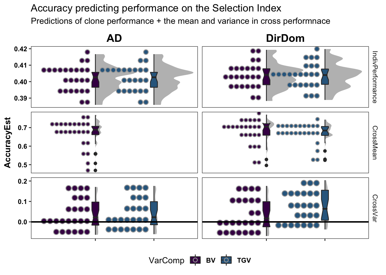
# + coord_cartesian(xlim = c(1.05, NA))The DirDom model is at least as good, if not better than AD. Suggest proceeding to consider only DirDom model genomic predictions.
Prediction accuracy estimates are in output/ (here) with filenames ending _predAccuracy.rds.
For details on the cross-validation scheme, see the article (and for even more, the corresponding supplemental documentation here).
Plots with breakdowns by traits
Standard cross-validation
Results, broken down by trait, for the “standard” 5 repeats of 5-fold cross-validation on the accuracy predicting individual-level performance. Contrast to the cross-mean and cross-variance predictions newly implemented and plotted further below.
stdcv_ad %>%
  unnest(accuracyEstOut) %>%
  select(-splits,-predVSobs,-seeds) %>%
  mutate(modelType="AD") %>%
  bind_rows(stdcv_dirdom %>%
              unnest(accuracyEstOut) %>%
              select(-splits,-predVSobs,-seeds) %>%
              mutate(modelType="DirDom")) %>%
  mutate(Trait=factor(Trait,levels=c("SELIND",blups$Trait)),
         predOf=factor(paste0(predOf,"_",modelType),levels=c("GEBV_AD","GETGV_AD","GEBV_DirDom","GETGV_DirDom"))) %>%
  ggplot(.,aes(x=predOf,y=Accuracy,fill=predOf,color=modelType)) +
  geom_boxplot(notch = TRUE, color='gray40') +
  scale_fill_manual(values = viridis::viridis(4)[1:4]) +
  scale_color_manual(values = viridis::viridis(4)[1:4]) +
  #geom_hline(yintercept = 0, color='black', size=0.8) +
  facet_grid(.~Trait) +
  labs(title="Accuracy predicting the performance of untested clones",
       subtitle="Standard 5-fold cross-validation") +
  theme_bw() +
  theme(axis.text.x = element_blank(),
        axis.title.x = element_blank(),
        strip.background = element_blank(),
        panel.grid.major = element_blank(),
        panel.grid.minor = element_blank(),
        legend.position='bottom',
        axis.text.y = element_text(face='bold'),
        axis.title.y = element_text(face='bold'),
        strip.text.x = element_text(face='bold'),
        plot.title = element_text(face='bold'),
        legend.title = element_text(face='bold'),
        legend.text = element_text(face='bold'),
        panel.spacing = unit(0.2, "lines"))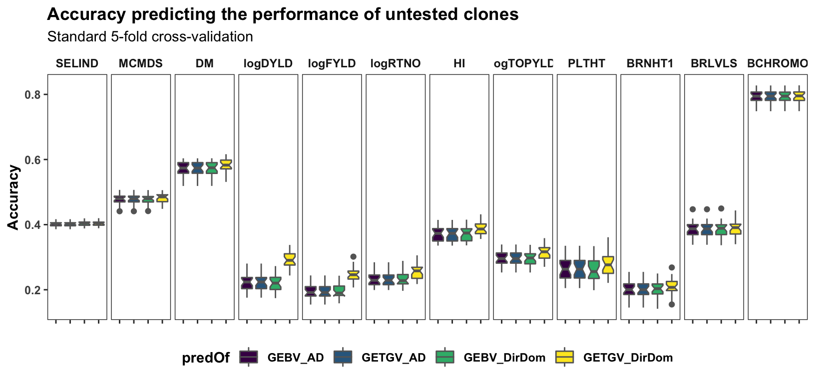
Parent-wise cross-validation
Cross-mean prediction accuracy
accuracy_ad$meanPredAccuracy %>%
  bind_rows(accuracy_dirdom$meanPredAccuracy) %>%
  select(-predVSobs) %>%
  mutate(Trait=factor(Trait,levels=c("SELIND",blups$Trait)),
         predOf=factor(paste0(predOf,"_",modelType),levels=c("MeanBV_AD","MeanTGV_AD","MeanBV_DirDom","MeanTGV_DirDom"))) %>%
  ggplot(.,aes(x=predOf,y=AccuracyEst,fill=predOf,color=modelType)) +
  geom_boxplot(notch = TRUE, color='gray40') +
  scale_fill_manual(values = viridis::viridis(4)[1:4]) +
  scale_color_manual(values = viridis::viridis(4)[1:4]) +
  geom_hline(yintercept = 0, color='black', size=0.8) +
  facet_grid(.~Trait) +
  labs(title="Accuracy predicting the mean performance of offspring from untested crosses",
       subtitle="5-fold 'parent-wise' cross-validation") +
  theme_bw() +
  theme(axis.text.x = element_blank(),
        axis.title.x = element_blank(),
        strip.background = element_blank(),
        panel.grid.major = element_blank(),
        panel.grid.minor = element_blank(),
        legend.position='bottom',
        axis.text.y = element_text(face='bold'),
        axis.title.y = element_text(face='bold'),
        strip.text.x = element_text(face='bold'),
        plot.title = element_text(face='bold'),
        legend.title = element_text(face='bold'),
        legend.text = element_text(face='bold'),
        panel.spacing = unit(0.2, "lines"))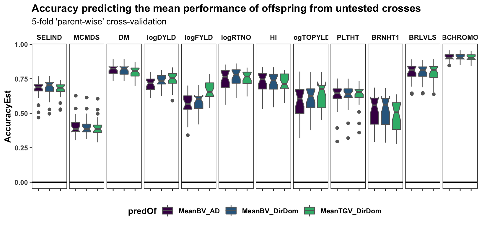
Cross-variance pred. accuracy
accuracy_ad$varPredAccuracy %>%
  bind_rows(accuracy_dirdom$varPredAccuracy) %>%
  select(-predVSobs) %>%
  filter(Trait1==Trait2) %>%
  mutate(Trait1=factor(Trait1,levels=c("SELIND",blups$Trait)),
         predOf=factor(paste0(predOf,"_",modelType),
                       levels=c("VarBV_AD","VarTGV_AD",
                                "VarBV_DirDom","VarTGV_DirDom"))) %>%
  ggplot(.,aes(x=predOf,y=AccuracyEst,fill=predOf,color=modelType)) +
  geom_boxplot(notch = TRUE,color='gray40') +
  scale_fill_manual(values = viridis::viridis(4)[1:4]) +
  scale_color_manual(values = viridis::viridis(4)[1:4]) +
  geom_hline(yintercept = 0, color='black', size=0.8) +
  facet_grid(.~Trait1) +
  labs(title="Accuracy predicting variance in performance among offspring of untested crosses",
       subtitle="5-fold 'parent-wise' cross-validation") +
  theme_bw() +
  theme(axis.text.x = element_blank(),
        axis.title.x = element_blank(),
        strip.background = element_blank(),
        panel.grid.major = element_blank(),
        panel.grid.minor = element_blank(),
        legend.position='bottom',
        axis.text.y = element_text(face='bold'),
        axis.title.y = element_text(face='bold'),
        strip.text.x = element_text(face='bold'),
        plot.title = element_text(face='bold'),
        legend.title = element_text(face='bold'),
        legend.text = element_text(face='bold'),
        panel.spacing = unit(0.2, "lines"))
Cross-co-variance pred. accuracy
accuracy_ad$varPredAccuracy %>%
  bind_rows(accuracy_dirdom$varPredAccuracy) %>%
  select(-predVSobs) %>%
  filter(Trait1!="SELIND",Trait2!="SELIND",
         Trait1!=Trait2) %>%
  mutate(Trait1=factor(Trait1,levels=c(blups$Trait)),
         Trait2=factor(Trait2,levels=c(blups$Trait)),
         predOf=factor(paste0(predOf,"_",modelType),
                       levels=c("VarBV_AD","VarTGV_AD",
                                "VarBV_DirDom","VarTGV_DirDom"))) %>%
  ggplot(.,aes(x=predOf,y=AccuracyEst,fill=predOf,color=modelType)) +
  geom_boxplot(notch = TRUE) +
  scale_fill_manual(values = viridis::viridis(4)[1:4]) +
  scale_color_manual(values = viridis::viridis(4)[1:4]) +
  geom_hline(yintercept = 0, color='gray40', size=0.6) +
  facet_wrap(~Trait1+Trait2,nrow=5) +
  labs(title="Accuracy predicting covariance in trait-trait performance within previously untested families",
       subtitle="5-fold 'parent-wise' cross-validation") +
theme_bw() +
  theme(axis.text.x = element_blank(),
        axis.title.x = element_blank(),
        strip.background = element_blank(),
        panel.grid.major = element_blank(),
        panel.grid.minor = element_blank(),
        legend.position='bottom',
        axis.text.y = element_text(face='bold'),
        axis.title.y = element_text(face='bold'),
        strip.text.x = element_text(face='bold'),
        plot.title = element_text(face='bold'),
        legend.title = element_text(face='bold'),
        legend.text = element_text(face='bold'),
        panel.spacing = unit(0.2, "lines"))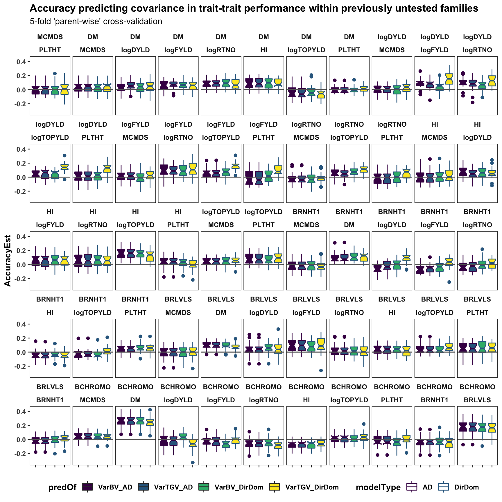
| Version | Author | Date |
|---|---|---|
| ba8527c | wolfemd | 2021-08-02 |
rm(list=ls())Genomic Predictions
After evaluating prediction accuracy, the genomic prediction step implements full-training dataset predictions and outputs tidy tables of selection criteria, including rankings on the selection index. For the sake of example, I selected 121 parents that were the union of parents ranking in the top 100 highest SELIND GEBV and/or GETGV as predicted by the DirDom and/or AD models. I predicted all 7381 crosses between these 121 pre-chosen parents and summarize those predictions below.
I find the accuracy results above compelling enough to focus on DirDom only below. In addition, below I focus on the selection index predictions (SELIND). Predictions of all component traits are also available. Feedback on presentation of results welcome!
- Download CSV of genomic predictions here: Standard genomic predictions of the individual GEBV and GETGV for all selection candidates. Use for parent and/or clone selection.
- Download CSV of genomic mate predictions here: Genomic predictions of cross means, variance and usefulness on the selection index and for component traits.
Genetic trends (and gain estimates)
Below, I start by looking at the genetic trends using selection index GEBV and GETGV of the individuals in the population, based on the DirDom model.
I highlight the top potential parents, for which all possible pairwise crosses are subsequently predicted and plotted.
# GBLUPs
### Two models AD and DirDom
gpreds_dirdom<-readRDS(file = here::here("output","genomicPredictions_ModelDirDom.rds"))
si_getgvs<-gpreds_dirdom$gblups[[1]] %>%
  filter(predOf=="GETGV") %>%
  select(GID,SELIND)

## IITA Germplasm Ages
ggcycletime<-readxl::read_xls(here::here("data","PedigreeGeneticGainCycleTime_aafolabi_01122020.xls")) %>%
  mutate(Year_Accession=as.numeric(Year_Accession))

# Need germplasmName field from raw trial data to match GEBV and cycle time
rawdata<-readRDS(here::here("output","IITA_ExptDesignsDetected_2021May10.rds"))
for_trend_plot<-si_getgvs %>%
  left_join(rawdata %>%
              distinct(germplasmName,GID)) %>%
  group_by(GID) %>%
  slice(1) %>%
  ungroup()
# table(ggcycletime$Accession %in% si_getgvs$germplasmName)
# FALSE  TRUE
#   193   614

for_trend_plot %<>%
  left_join(.,ggcycletime %>%
              rename(germplasmName=Accession) %>%
              mutate(Year_Accession=as.numeric(Year_Accession))) %>%
  mutate(Year_Accession=case_when(grepl("2013_|TMS13",germplasmName)~2013,
                                  grepl("TMS14",germplasmName)~2014,
                                  grepl("TMS15",germplasmName)~2015,
                                  grepl("TMS18",germplasmName)~2018,
                                  !grepl("2013_|TMS13|TMS14|TMS15|TMS18",germplasmName)~Year_Accession))

# Declare the "eras" as PreGS\<2012 and GS\>=2013.
for_trend_plot %<>%
  filter(Year_Accession>2012 | Year_Accession<2005)
for_trend_plot %<>%
  mutate(GeneticGroup=ifelse(Year_Accession>=2013,"GS","PreGS"))

plottheme<-theme_bw() +
  theme(axis.text.x = element_blank(),
        axis.title.x = element_blank(),
        strip.background = element_blank(),
        panel.grid.major = element_blank(),
        panel.grid.minor = element_blank(),
        legend.position='bottom',
        axis.text.y = element_text(face='bold'),
        axis.title.y = element_text(face='bold'),
        strip.text.x = element_text(face='bold'),
        plot.title = element_text(face='bold'),
        legend.title = element_text(face='bold'),
        legend.text = element_text(face='bold'),
        panel.spacing = unit(0.2, "lines"))
First, for the IITA population, I use historical data on age of clones to perform a regression of GETGV on year-cloned compared the post 2012 (GS) to pre-GS era. The plot below shows the GETGV (y-axis) versus the year each accession was cloned.
for_trend_plot %>%
  select(GeneticGroup,GID,Year_Accession,SELIND) %>%
  ggplot(.,aes(x=Year_Accession,y=SELIND,color=GeneticGroup)) +
  geom_point(size=1.25) +
  geom_smooth(method=lm, se=TRUE, size=1.5) +
  plottheme + theme(panel.grid.major = element_line()) +
  scale_color_viridis_d() +
  labs(title = "Selection Index GETGV vs. Accession Age by 'era' [GS vs. PreGS]",
subtitle = "SI GETGV from modelType='DirDom'") 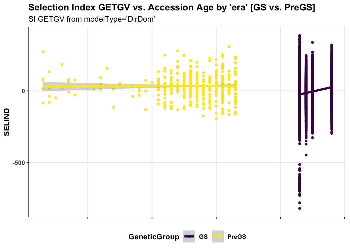
Next, some fancy boxplot / half-violin plots to compare the distribution of GETGV across the cycles.
si_getgvs %>%
  mutate(GeneticGroup=case_when(grepl("2013_|TMS13",GID)~"C1",
                                grepl("TMS14",GID)~"C2",
                                grepl("TMS15",GID)~"C3",
                                grepl("TMS18",GID)~"C4",
                                !grepl("2013_|TMS13|TMS14|TMS15|TMS18",GID)~"PreGS"),
         GeneticGroup=factor(GeneticGroup,levels = c("PreGS","C1","C2","C3","C4"))) %>%
  ggplot(.,aes(x=GeneticGroup,y=SELIND,fill=GeneticGroup)) +
  ggdist::stat_halfeye(adjust=0.5,.width = 0,fill='gray',width=0.75) +
  geom_boxplot(width=0.12,notch = TRUE) +
  ggdist::stat_dots(side = "left",justification = 1.1,
                    binwidth = 0.03,dotsize=0.6) +
  plottheme +
  scale_fill_viridis_d()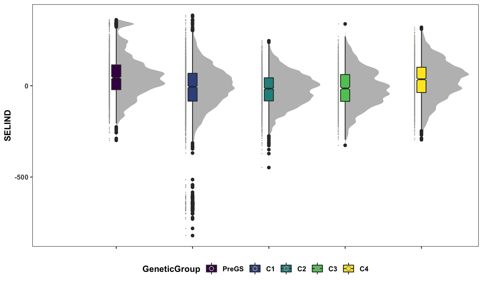
Lastly, for continuity sake, barplots of the mean +/- std. error of GEBV across the cycles.
si_gebvs<-gpreds_dirdom$gblups[[1]] %>%
  filter(predOf=="GEBV") %>%
  select(GID,SELIND) %>%
  mutate(GeneticGroup=case_when(grepl("2013_|TMS13",GID)~"C1",
                                  grepl("TMS14",GID)~"C2",
                                  grepl("TMS15",GID)~"C3",
                                  grepl("TMS18",GID)~"C4",
                                  !grepl("2013_|TMS13|TMS14|TMS15|TMS18",GID)~"PreGS"),
         GeneticGroup=factor(GeneticGroup,levels = c("PreGS","C1","C2","C3","C4")))
si_gebvs %>%
  group_by(GeneticGroup) %>%
  summarize(meanGEBV=mean(SELIND),
            stdErr=sd(SELIND)/sqrt(n()),
            upperSE=meanGEBV+stdErr,
            lowerSE=meanGEBV-stdErr) %>%
  ggplot(.,aes(x=GeneticGroup,y=meanGEBV,fill=GeneticGroup)) +
  geom_bar(stat = 'identity', color='gray60', size=1.25) +
  geom_linerange(aes(ymax=upperSE,
                     ymin=lowerSE), color='gray60', size=1.25) +
  #facet_wrap(~Trait,scales='free_y', ncol=1) +
  theme_bw() +
  geom_hline(yintercept = 0, size=1.15, color='black') +
  plottheme +
  scale_fill_viridis_d() +
  labs(x=NULL,y="Mean GEBVs",
       title="Mean +/- Std. Error Selection Index GEBV by Cycle")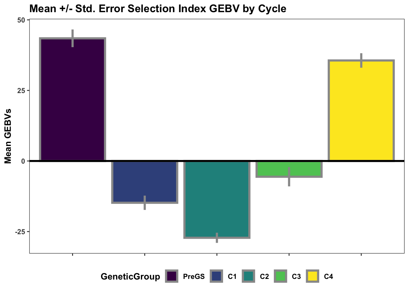
| Version | Author | Date |
|---|---|---|
| ba8527c | wolfemd | 2021-08-02 |
Parent selection
library(tidyverse); library(magrittr); library(ggdist)
# crossPreds<-readRDS(file = here::here("output","genomicMatePredictions_top121parents_ModelDirDom.rds"))
# crossPreds<-crossPreds$tidyPreds[[1]]
crossPreds<-read.csv(here::here("output","genomicMatePredictions_top121parents_ModelAD.csv"), stringsAsFactors = F, header = T)
I predicted 7381 crosses of 121 parents originally selected as the union of elite parents predicted by both DirDom and AD models. So not all these parents are the absolute top in terms of SI GETGV and the DirDom model, which I will plot below. Since I made the predictions for those extra parents, they are plotted here.
for_selected_plot<-si_getgvs %>%
  mutate(GeneticGroup=case_when(grepl("2013_|TMS13",GID)~"C1",
                                grepl("TMS14",GID)~"C2",
                                grepl("TMS15",GID)~"C3",
                                grepl("TMS18",GID)~"C4",
                                !grepl("2013_|TMS13|TMS14|TMS15|TMS18",GID)~"PreGS"))
for_selected_plot %>%
  mutate(Cycle="AllGermplasm") %>%
  bind_rows(for_selected_plot %>%
              filter(GID %in% union(crossPreds$sireID,crossPreds$damID)) %>%
              mutate(Cycle="SelectedParents")) %>%
  mutate(Cycle=factor(Cycle,levels = c("AllGermplasm","SelectedParents")),
         GeneticGroup=factor(GeneticGroup,levels = c("PreGS","C1","C2","C3","C4"))) %>%
  ggplot(.,aes(x=Cycle,y=SELIND,fill=Cycle)) +
  ggdist::stat_halfeye(adjust=0.5,.width = 0,fill='gray',width=0.75) +
  geom_boxplot(width=0.09,notch = TRUE) +
  ggdist::stat_dots(aes(color=GeneticGroup),side = "left",justification = 1.1,dotsize=.8) +
  scale_fill_viridis_d() + scale_color_viridis_d() +
  plottheme +
  labs(title="Distribution of selection index GETGV in parents selected for mate predictions",
       subtitle="compared to the overall population")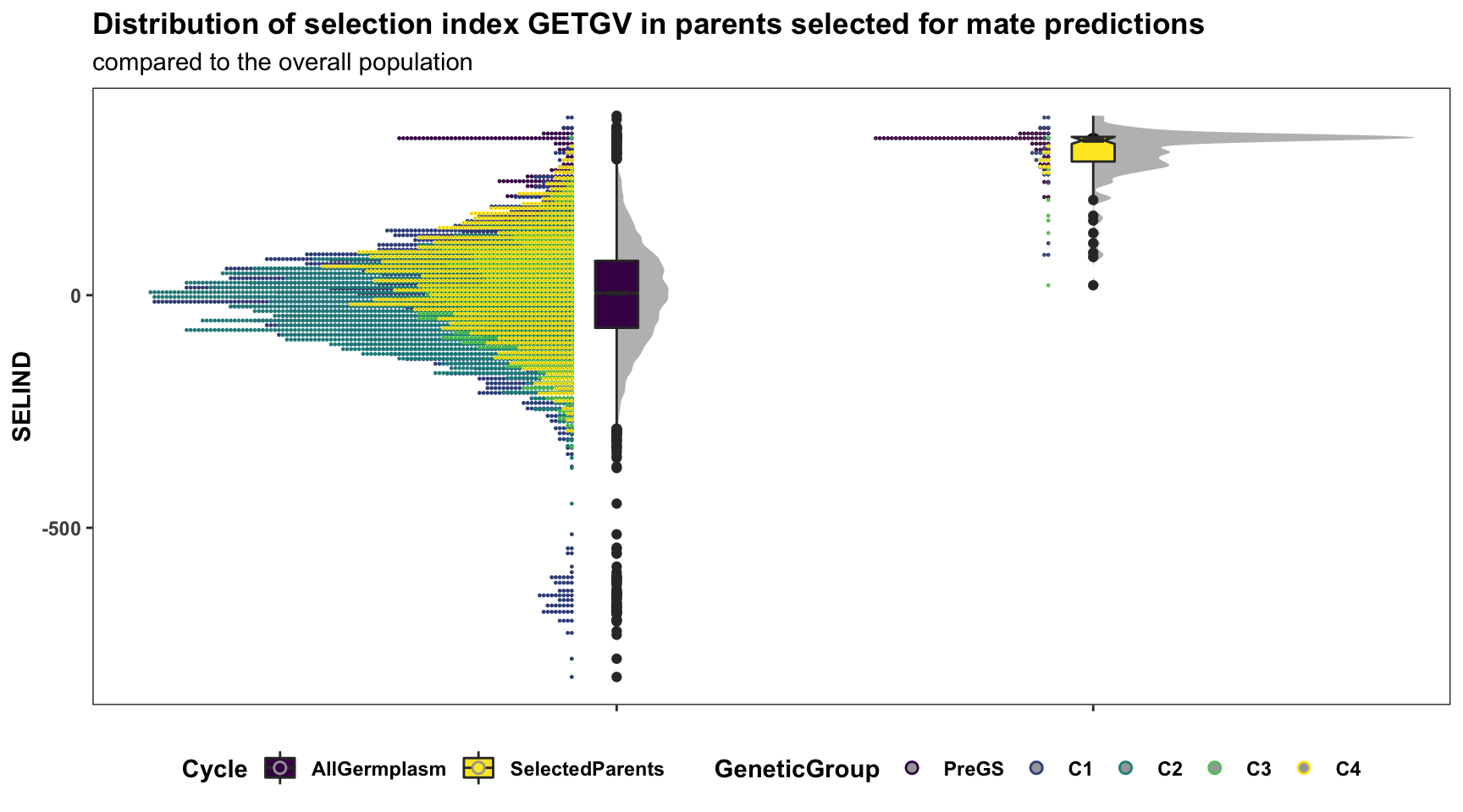
| Version | Author | Date |
|---|---|---|
| ba8527c | wolfemd | 2021-08-02 |
Genomic mate selection
library(tidyverse); library(magrittr); library(ggdist)
# crossPreds<-readRDS(file = here::here("output","genomicMatePredictions_top121parents_ModelDirDom.rds"))
# crossPreds<-crossPreds$tidyPreds[[1]]
crossPreds<-read.csv(here::here("output","genomicMatePredictions_top121parents_ModelAD.csv"), stringsAsFactors = F, header = T)
forplot<-crossPreds %>%
  filter(Trait=="SELIND") %>%
  select(sireID,damID,CrossGroup,predOf,predMean,predSD)

cross_group_order<-crossPreds %>%
  filter(Trait=="SELIND") %>%
  distinct(sireGroup,damGroup) %>%
  mutate(sireGroup=factor(sireGroup,levels=c("PreGS","C1","C2","C3","C4")),
         damGroup=factor(damGroup,levels=c("PreGS","C1","C2","C3","C4"))) %>%
  arrange(desc(sireGroup),desc(damGroup)) %>%
  mutate(CrossGroup=paste0(sireGroup,"x",damGroup)) %$%
  CrossGroup

intensity<-function(propSel){ dnorm(qnorm(1-propSel))/propSel } # standardized selection intensity
stdSelInt=intensity(0.05); # stdSelInt [1] 2.062713
# qnorm(0.95); # [1] 1.644854
forplot %<>%
  mutate(predUsefulness=predMean+(predSD*stdSelInt),
         CrossGroup=factor(CrossGroup,levels=c(cross_group_order)))
The standard budget for genotyping has been 2500 new clones per year.
Suppose we choose to create 50 families of 50 siblings each, from the the 7381 predicted crosses.
Quick digression: The input file has a pre-computed predUsefulness variable. I used stdSelInt=2.67 when making the predictions with the predictCrosses() function, but that corresponds to selecting the top 1% of each family. For a family of 50, the top 1% means only a single clone per family. In retrospect, I have decided to re-compute the predUsefulness targeting selection of the top 5% (or top 5 offspring) from each family. This corresponds to using stdSelInt = 2.0627128 and a selection threshold std. deviation of 1.6448536.
Crosses may be of interest for their predicted \(UC_{parent}\) (predOf=="BV") and/or \(UC_{variety}\) (predOf=="TGV").
Each crossing nursery needs to produce both new exceptional parents and elite candidate cultivars. These will not necessarily be the same individuals or come from the same crosses.
# forplot %>%
#   select(-predMean,-predSD) %>%
#   spread(predOf,predUsefulness) %$%
#   cor(BV,TGV)
# [1] 0.999988
# The correlation between predUC BV and TGV is extremely high


# forplot %>%
#   group_by(predOf) %>%
#   slice_max(order_by = predUsefulness, n = 50) %>% ungroup() %>%
#   distinct(sireID,damID) %>% nrow() # 50
# Also, the exact same 50 are ranked top predUC
In this case, the same 50 crosses are best for both \(UC_{parent}\) (predOf=="BV") and \(UC_{variety}\) (predOf=="TGV").
First, display the entire set of predicted crosses, ranked by their selection index \(UC^{SI}_{variety}\). This will be more clear in the next plots with fewer families: the x-axis is simply the descending rank of predicted \(UC^{SI}_{variety}\) for each cross. The y-axis shows the predicted mean (dot) and distribution quantiles (linerange) based on the predicted mean and standard deviation of each cross. Crosses are color coded according to the “genetic group” of the parents.
forplot %>%
  filter(predOf=="TGV") %>%
  #slice_max(order_by = predUsefulness, n = 100) %>%
  arrange(desc(predUsefulness)) %>%
  mutate(Rank=1:nrow(.)) %>%
  ggplot(aes(x = Rank, dist = "norm",
             arg1 = predMean, arg2 = predSD,
             fill=CrossGroup, color=CrossGroup),
         alpha=0.5) +
  stat_dist_pointinterval() +
  #stat_dist_gradientinterval(n=50) +
  scale_fill_viridis_d() + scale_color_viridis_d() +
  plottheme + theme() +
  labs(x = paste0("Cross Rank ",expression(bold("UC"["variety"]~" (TGV)"))),
       y = "Selection Index GETGV",
       title = "Predicted distribution (mean and variability) of all crosses")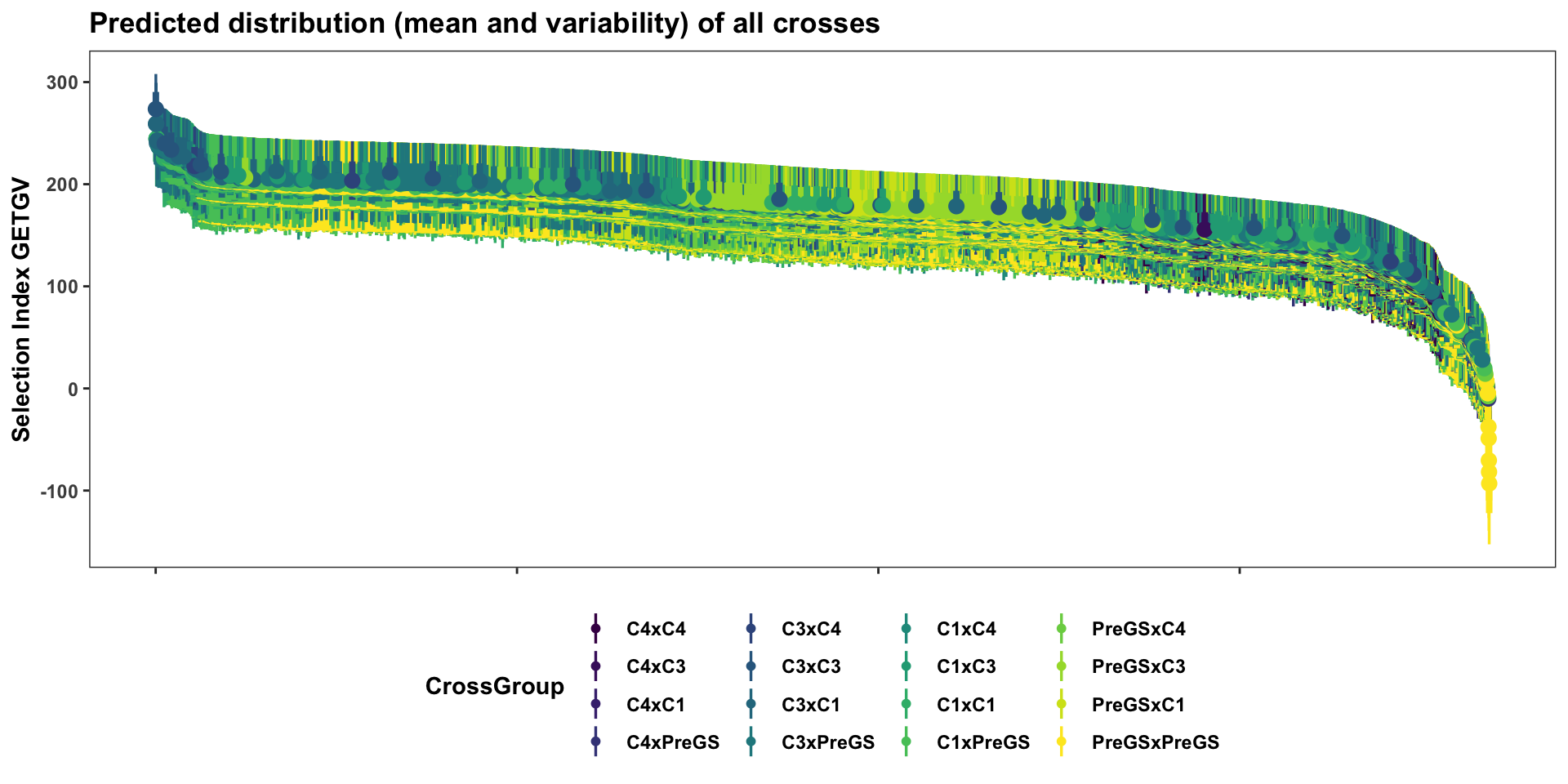
Next, sub
forplot %>%
  filter(predOf=="TGV") %>%
  slice_max(order_by = predUsefulness, n = 50) %>%
  arrange(desc(predUsefulness)) %>%
  mutate(Rank=1:nrow(.)) %>%
    ggplot(aes(x = Rank, dist = "norm",
               arg1 = predMean, arg2 = predSD,
               fill=CrossGroup, color=CrossGroup),
           alpha=0.5) +
    stat_dist_gradientinterval(n=100) +
    scale_fill_viridis_d() + scale_color_viridis_d() +
  plottheme + theme(axis.text.x = element_text(face='bold'),
                    axis.title.x = element_text(face = 'bold')) +
  labs(x = expression(bold("Rank on SELIND - UC"["variety"])),
       y = "Selection Index GETGV",
       title = "Predicted distribution of the top 50 crosses")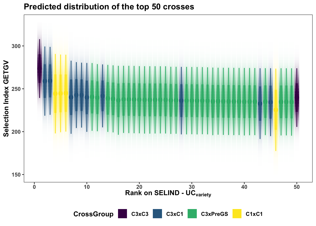
| Version | Author | Date |
|---|---|---|
| ba8527c | wolfemd | 2021-08-02 |
The best 5 crosses to make:
forplot %>%
  filter(predOf=="TGV") %>%
  slice_max(order_by = predUsefulness, n = 5) %>% rmarkdown::paged_table()
Interestingly (?) no cross of C4 (TMS18) clones are yet recommended (in the top 50) on this ranking. The highest rank C4 cross is the 214th from top (see below) along with two other TMS18 x TMS15 crosses.
forplot %>%
  filter(predOf=="TGV") %>%
  arrange(desc(predUsefulness)) %>%
  mutate(Rank=1:nrow(.)) %>%
  filter(grepl("C4",CrossGroup)) %>% slice(1:10) %>%
  rmarkdown::paged_table()
In this last plot, the area under the top 5% of each crosses predicted distribution is highlighted. The mean of individuals from under the highlighted area is the \(UC_{variety}\). There are also 50 dots for each cross illustrating the hypothetical outcome of creating 50 progeny.
forplot %>%
  filter(predOf=="TGV") %>%
  slice_max(order_by = predUsefulness, n = 50) %>%
  arrange(desc(predUsefulness)) %>%
  mutate(Rank=1:nrow(.)) %>%
  ggplot(aes(x = Rank, dist = "norm",
             arg1 = predMean, arg2 = predSD,
             fill = CrossGroup,
             label = CrossGroup)) +
  stat_dist_gradientinterval(n=100,side='top',position = "dodgejust",
                         aes(fill = stat(y < (arg1+arg2*qnorm(0.95))))) +
  stat_dist_dotsinterval(n=50,side='both',position = "dodgejust",
                         aes(fill = stat(y < (arg1+arg2*qnorm(0.95))))) +
  scale_fill_viridis_d() + scale_color_viridis_d() +
  plottheme + theme(axis.text.x = element_text(face='bold'),
                    axis.title.x = element_text(face = 'bold'),
                    legend.position = 'none') +
  labs(x = expression(bold("Rank on SELIND - UC"["variety"])),
       y = "Selection Index GETGV",
       title = "Predicted distribution of the top 50 crosses")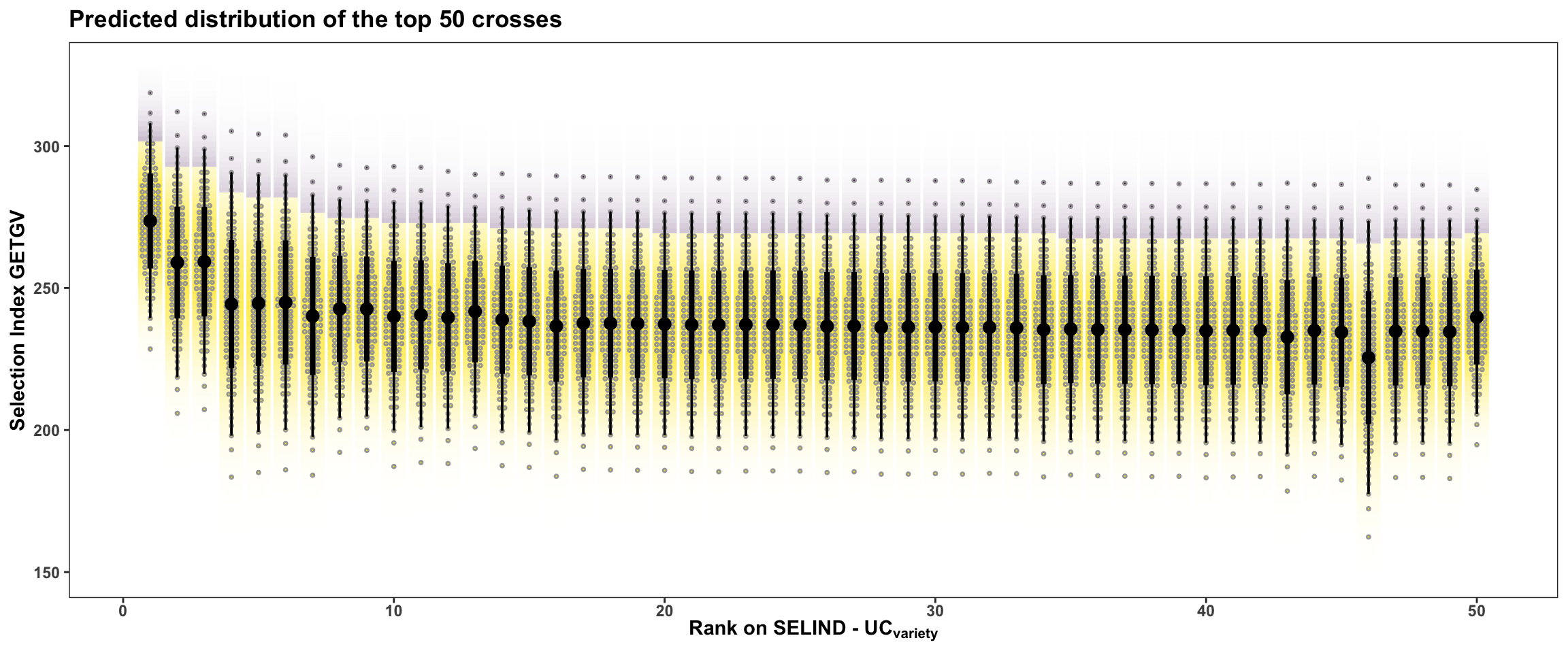
Or for more clarity, just the top 5 crosses:
forplot %>%
  filter(predOf=="TGV") %>%
  slice_max(order_by = predUsefulness, n = 5) %>%
  arrange(desc(predUsefulness)) %>%
  mutate(Rank=1:nrow(.)) %>%
  ggplot(aes(y = Rank, dist = "norm",
             arg1 = predMean, arg2 = predSD,
             label = paste0(sireID,"\n x ",damID)),
         alpha=0.5) +
  stat_dist_dotsinterval(n=50,side='top',position = "dodgejust",scale=0.85,
                         aes(fill = stat(x < (arg1+arg2*qnorm(0.95))))) +
  stat_dist_halfeye(position = "dodgejust",scale=1.25, alpha=0.5,
                    aes(fill = stat(x < (arg1+arg2*qnorm(0.95))))) +
  geom_label(aes(x=predMean),size=3) +
  scale_fill_viridis_d() + scale_color_viridis_d() +
  plottheme + theme(axis.text.x = element_text(face='bold'),
                    axis.title.x = element_text(face = 'bold'),
                    legend.position = 'none') +
  labs(y = expression(bold("Rank on SELIND - UC"["variety"])),
       x = "Selection Index GETGV",
       title = "Predicted distribution of the top 5 crosses")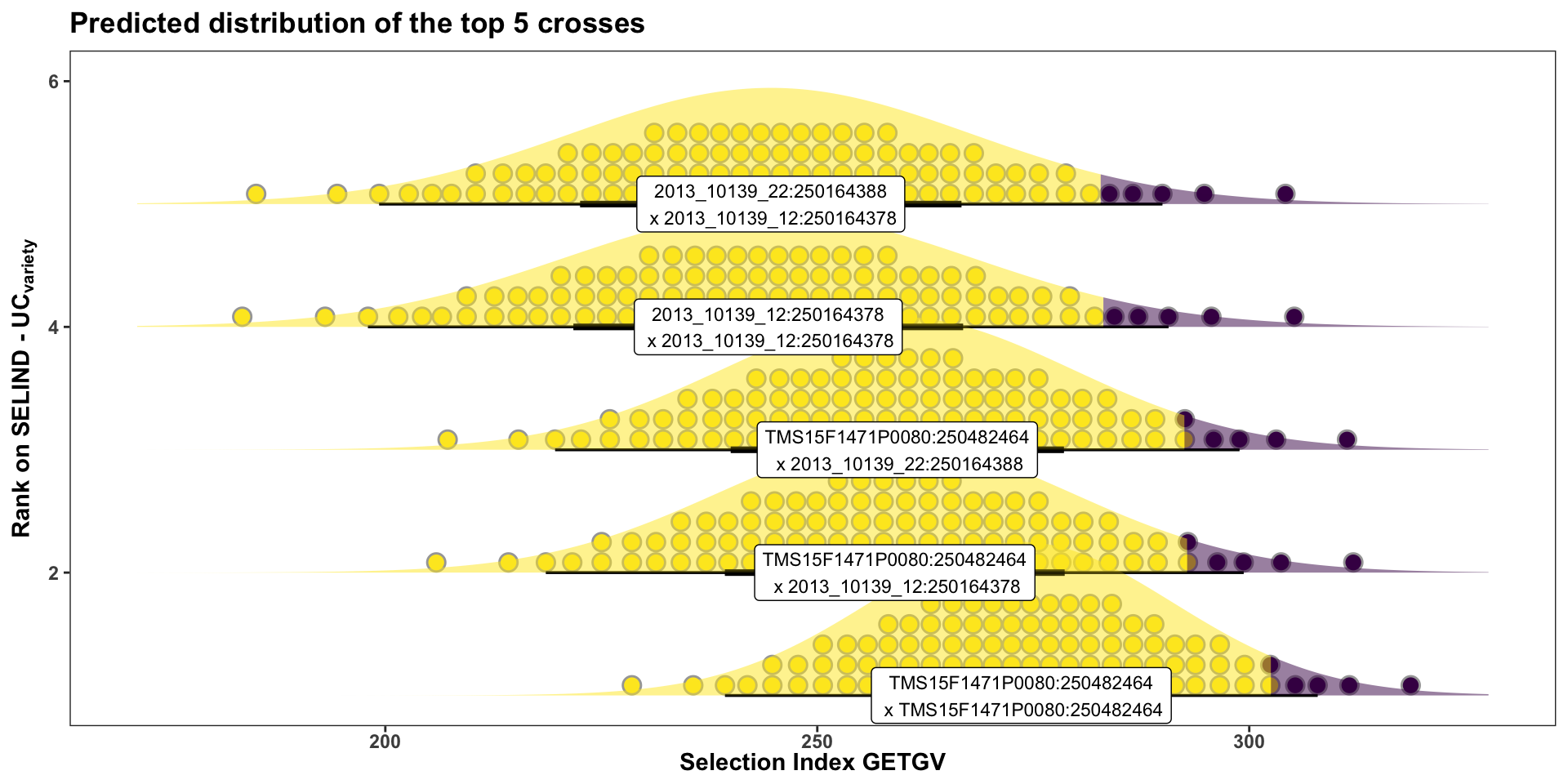
| Version | Author | Date |
|---|---|---|
| ba8527c | wolfemd | 2021-08-02 |
Table of Top 50 Crosses: 2 rows for each cross, one for predOf=="BV" one for predOf=="TGV".
- Download the CSV for the top 50 crosses and their selection index means, SDs and UC here or
- Download the complete CSV of ALL genomic mate predictions here: for all crosses and both SELIND and component trait predictions.
top50crosses<-forplot %>%
  group_by(predOf) %>%
  slice_max(order_by = predUsefulness, n = 50) %>%
  ungroup()
top50crosses %>%
  write.csv(.,file = here::here("output","top50crosses.csv"), row.names = F)
top50crosses %>%
  rmarkdown::paged_table()
Optimize marker density for speed
Test whether marker density can be reduced to save compute time (enabling us to predict more crosses) without sacrificing prediction accuracy. Use both standard and parent-wise cross-validation and LD-based pruning of markers. Analyses are documented here.
Selection index
library(ggdist)
accuracy<-list.files(path = here::here("output")) %>%
  grep("_predAccuracy",.,value = T) %>%
  grep("_1Mb_50kb_pt|cvDirDom_5rep5fold_|stdcv_DirDom_",.,value = T) %>%
  tibble(Filename=.) %>%
  mutate(CVtype=ifelse(grepl("stdcv",Filename),"StandardCV","ParentwiseCV"),
         Filter=gsub("_predAccuracy.rds","",Filename),
         Filter=gsub("cvDirDom_|stdcvDirDom_","",Filter),
         Filter=ifelse(Filter %in% c("5rep5fold","stdcv_DirDom"),"50snp_25snp_pt98",Filter),
         results=map(Filename,~readRDS(here::here("output",.))))
accuracy %<>%
  mutate(results=map2(CVtype,results,function(CVtype,results){
    if(CVtype=="ParentwiseCV"){
      out<-results$meanPredAccuracy %>%
        bind_rows(results$meanPredAccuracy) %>%
        filter(Trait=="SELIND") %>%
        mutate(VarComp=gsub("Mean","",predOf),
               predOf="CrossMean") %>%
        bind_rows(results$varPredAccuracy %>%
                    bind_rows(results$varPredAccuracy) %>%
                    filter(Trait1=="SELIND") %>%
                    rename(Trait=Trait1) %>%
                    select(-Trait2) %>%
                    mutate(VarComp=gsub("Var","",predOf),
                           predOf="CrossVar")) %>%
        select(-predVSobs) }
    if(CVtype=="StandardCV"){
      out<-results %>%
        select(-splits,-seeds) %>%
        unnest(accuracyEstOut) %>%
        select(-predVSobs) %>%
        filter(Trait=="SELIND") %>%
        rename(Repeat=repeats,Fold=id,VarComp=predOf,AccuracyEst=Accuracy) %>%
        mutate(Repeat=paste0("Repeat",Repeat),
               VarComp=gsub("GE","",VarComp),
               predOf="IndivPerformance",
               modelType="DirDom")
    }
    return(out) }))
accuracy %<>%
left_join(tribble(~Filter,~Nsnp,~ParentwiseRuntime,
"50snp_25snp_pt98",34981,34.5,
"1Mb_50kb_pt9",20645,10.65,
"1Mb_50kb_pt8",15342,7.14,
"1Mb_50kb_pt6",9501,5.28,
"1Mb_50kb_pt5",7412,4.42)) %>%
unnest(results)
accuracy %<>%
mutate(predOf=factor(predOf,levels=c("IndivPerformance","CrossMean","CrossVar")),
VarComp=factor(VarComp,levels=c("BV","TGV")))
plottheme<-theme(axis.text.x = element_blank(),
axis.title.x = element_blank(),
strip.background = element_blank(),
panel.grid.major = element_blank(),
panel.grid.minor = element_blank(),
axis.title = element_text(face='bold',color = 'black'),
strip.text.x = element_text(face='bold',color='black',size=14),
axis.text.y = element_text(face = 'bold',color='black'),
legend.text = element_text(face='bold'),
legend.position = 'bottom')accuracy %>%
ggplot(.,aes(x=VarComp,y=AccuracyEst,fill=VarComp)) +
ggdist::stat_halfeye(adjust=0.5,.width = 0,fill='gray',width=0.75) +
geom_boxplot(width=0.12,notch = TRUE) +
ggdist::stat_dots(side = "left",justification = 1.1,dotsize=0.6)+
theme_bw() +
scale_fill_manual(values = viridis::viridis(4)[1:2]) +
geom_hline(data = accuracy %>% distinct(predOf) %>% filter(predOf=="CrossVar") %>% mutate(yint=0),
aes(yintercept = yint), color='black', size=0.9) +
plottheme +
facet_grid(predOf~Nsnp,scales = 'free') +
labs(title="Accuracy predicting performance on the Selection Index",
subtitle="Versus number of SNPs remaining after LD-pruning") 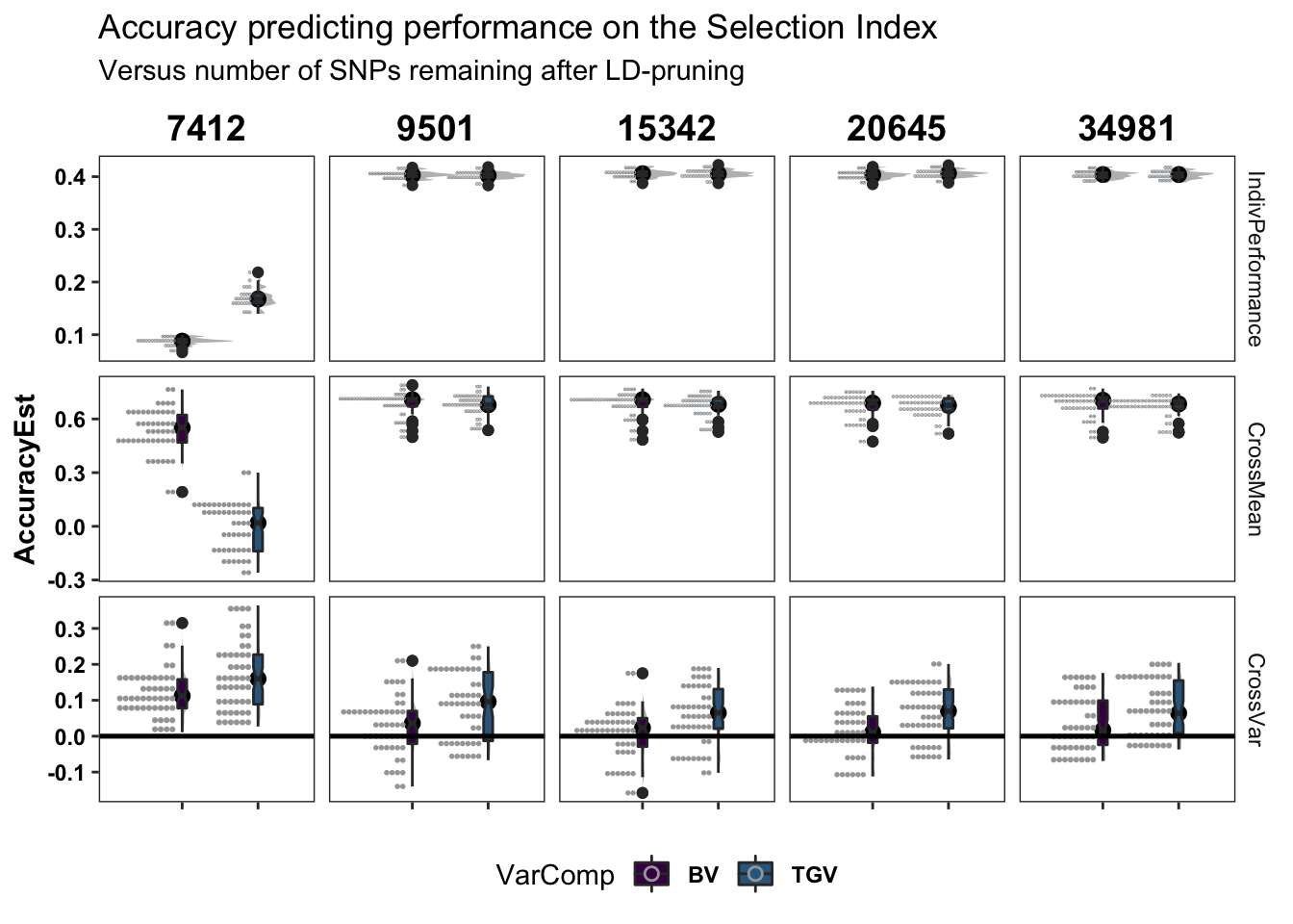
# + coord_cartesian(xlim = c(1.05, NA))Turn it into a line lot with Nsnp on x-axis. Lines grouped by Rep-Fold-VarComp
accuracy %>%
  ggplot(.,aes(x=Nsnp,y=AccuracyEst,color=VarComp,group=paste0(Repeat,"_",Fold,"_",VarComp))) +
  geom_point() + geom_line(alpha=0.85) +
  #ggdist::stat_halfeye(adjust=0.5,.width = 0,fill='gray',width=0.75) +
  #geom_boxplot(width=0.12,notch = TRUE) +
  #ggdist::stat_dots(side = "left",justification = 1.1,dotsize=0.6)+
  theme_bw() +
  scale_color_manual(values = viridis::viridis(4)[1:2]) +
  geom_hline(data = accuracy %>% distinct(predOf) %>% filter(predOf=="CrossVar") %>% mutate(yint=0),
             aes(yintercept = yint), color='black', size=0.9) +
  plottheme + theme(axis.text.x = element_text(face='bold'),
                    axis.title.x = element_text(face='bold')) +
  facet_grid(predOf~.,scales = 'free') +
  labs(title="Accuracy predicting performance on the Selection Index",
subtitle="Versus number of SNPs remaining after LD-pruning") 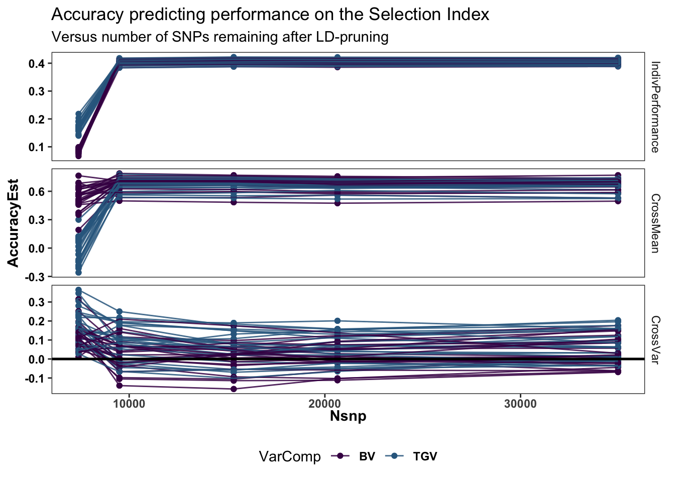
# + coord_cartesian(xlim = c(1.05, NA))Cross variance accuracy seems to up !?? while CrossMean and Indiv Accuracy suddenly drop at the lowest level?
Zoom in….
accuracy %>% filter(predOf!="IndivPerformance",Nsnp<20000) %>% droplevels %>%
  ggplot(.,aes(x=Nsnp,y=AccuracyEst,color=VarComp,group=paste0(Repeat,"_",Fold,"_",VarComp))) +
  geom_point(size=1.5) + geom_line(size=1.25,alpha=0.8) +
  #ggdist::stat_halfeye(adjust=0.5,.width = 0,fill='gray',width=0.75) +
  #geom_boxplot(width=0.12,notch = TRUE) +
  #ggdist::stat_dots(side = "left",justification = 1.1,dotsize=0.6)+
  theme_bw() +
  scale_color_manual(values = viridis::viridis(4)[1:2]) +
  geom_hline(data = accuracy %>% distinct(predOf) %>% filter(predOf=="CrossVar") %>% mutate(yint=0),
             aes(yintercept = yint), color='black', size=1.5) +
  plottheme + theme(axis.text.x = element_text(face='bold'),
                    axis.title.x = element_text(face='bold')) +
  facet_grid(predOf~.,scales = 'free') +
  labs(title="Accuracy predicting performance on the Selection Index",
subtitle="Versus number of SNPs remaining after LD-pruning") 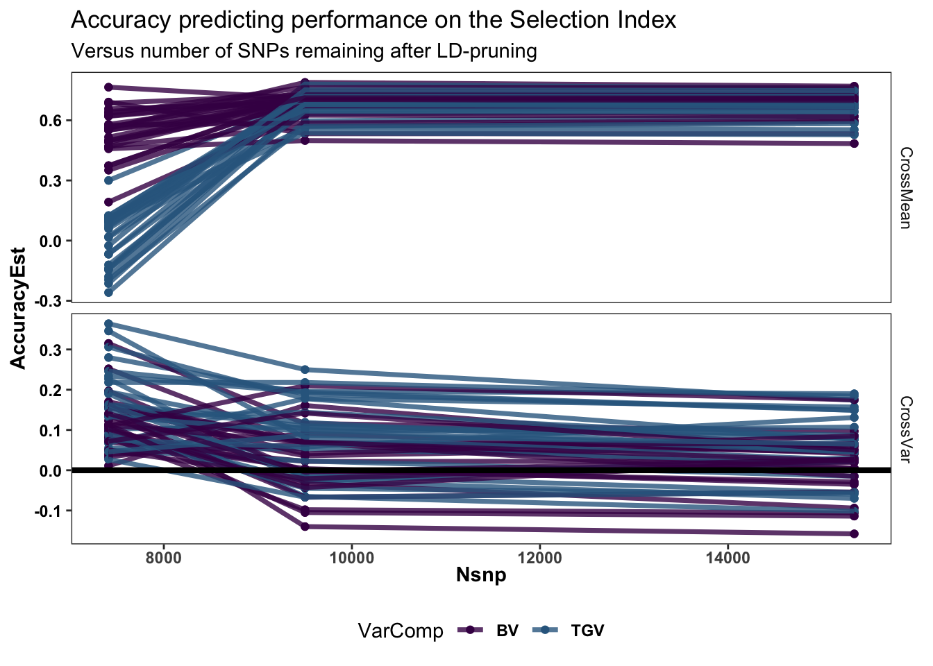
# + coord_cartesian(xlim = c(1.05, NA))predVSobs plots
accuracy<-list.files(path = here::here("output")) %>%
  grep("_predAccuracy",.,value = T) %>%
  grep("_1Mb_50kb_pt|cvDirDom_5rep5fold_|stdcv_DirDom_",.,value = T) %>%
  tibble(Filename=.) %>%
  mutate(CVtype=ifelse(grepl("stdcv",Filename),"StandardCV","ParentwiseCV"),
         Filter=gsub("_predAccuracy.rds","",Filename),
         Filter=gsub("cvDirDom_|stdcvDirDom_","",Filter),
         Filter=ifelse(Filter %in% c("5rep5fold","stdcv_DirDom"),"50snp_25snp_pt98",Filter),
         results=map(Filename,~readRDS(here::here("output",.))))
accuracy %<>%
  mutate(processed=map2(CVtype,results,function(CVtype,results){
    if(CVtype=="ParentwiseCV"){
      out<-results$meanPredAccuracy %>%
        bind_rows(results$meanPredAccuracy) %>%
        filter(Trait=="SELIND") %>%
        mutate(VarComp=gsub("Mean","",predOf),
               predOf="CrossMean") %>%
        bind_rows(results$varPredAccuracy %>%
                    bind_rows(results$varPredAccuracy) %>%
                    filter(Trait1=="SELIND") %>%
                    rename(Trait=Trait1) %>%
                    select(-Trait2) %>%
                    mutate(VarComp=gsub("Var","",predOf),
                           predOf="CrossVar")) %>%
        select(-predVSobs) }
    if(CVtype=="StandardCV"){
      out<-results %>%
        select(-splits,-seeds) %>%
        unnest(accuracyEstOut) %>%
        select(-predVSobs) %>%
        filter(Trait=="SELIND") %>%
        rename(Repeat=repeats,Fold=id,VarComp=predOf,AccuracyEst=Accuracy) %>%
        mutate(Repeat=paste0("Repeat",Repeat),
               VarComp=gsub("GE","",VarComp),
               predOf="IndivPerformance",
               modelType="DirDom")
    }
return(out) }))forplot<-accuracy %>%
filter(CVtype=="ParentwiseCV") %>%
select(CVtype,Filter,results) %>%
mutate(results=map(results,~.$varPredAccuracy %>%
filter(Trait1=="SELIND") %>%
select(Repeat,Fold,predOf,predVSobs) %>%
unnest(predVSobs))) %>%
left_join(tribble(~Filter,~Nsnp,~ParentwiseRuntime,
"50snp_25snp_pt98",34981,34.5,
"1Mb_50kb_pt9",20645,10.65,
"1Mb_50kb_pt8",15342,7.14,
"1Mb_50kb_pt6",9501,5.28,
"1Mb_50kb_pt5",7412,4.42)) %>%
unnest(results) %>%
mutate(predOf=factor(predOf,levels=c("VarBV","VarTGV")))
plottheme<-theme(axis.text.x = element_blank(),
axis.title.x = element_blank(),
strip.background = element_blank(),
panel.grid.major = element_blank(),
panel.grid.minor = element_blank(),
axis.title = element_text(face='bold',color = 'black'),
strip.text.x = element_text(face='bold',color='black',size=14),
axis.text.y = element_text(face = 'bold',color='black'),
legend.text = element_text(face='bold'),
legend.position = 'bottom')Plot the predicted vs. obsered cross variances (on the SELIND) to see if there is anything informative about the lowest SNP set level….
forplot %>%
  ggplot(.,aes(x=predVar,y=obsVar,size=famSize,color=predOf)) +
  geom_point(alpha=0.6) +
  geom_abline(slope=1,color='darkred') +
  theme_bw() +
  scale_color_manual(values = viridis::viridis(4)[1:2]) +
  plottheme +
  facet_wrap(predOf~Nsnp,scales = 'free',nrow=2) +
  labs(title="Predicted vs. observed cross variances (selection index)",
subtitle="Versus number of SNPs remaining after LD-pruning") 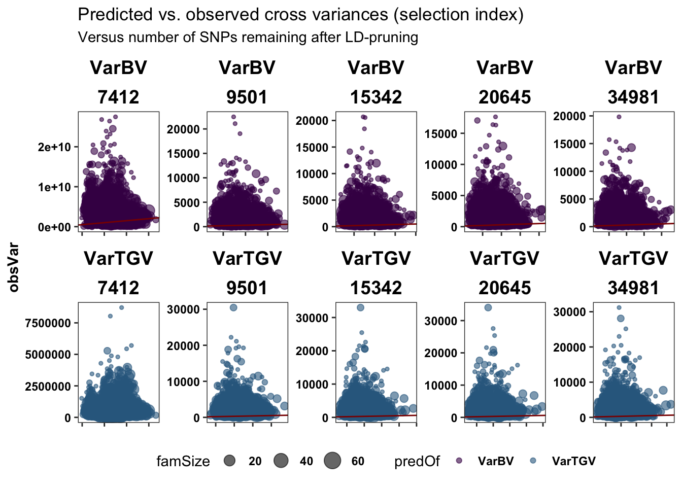
# + coord_cartesian(xlim = c(1.05, NA))Nothing looks special at Nsnp=7412, but the scale is off…
Next, make correlation matrices among the obsVar (and subsequently the predVar) at different Nsnp levels.
Data.frame below shows two matrices, one for each VarBV and VarTGV (but the result they show is pretty much the same)…
# obsVar cors
forplot %>%
  select(-predVar,-ParentwiseRuntime,-Filter) %>%
  pivot_wider(names_from = "Nsnp",
              names_prefix = "Nsnp",
              values_from = "obsVar") %>%
  select(predOf,contains("Nsnp")) %>%
  nest(data=-predOf) %>%
  mutate(data=map(data,~cor(.,use = 'pairwise.complete.obs') %>%
              round(.,2) %>% as.data.frame %>% rownames_to_column(var = "Nsnp"))) %>%
  unnest(data)
# A tibble: 10 × 7
predOf Nsnp Nsnp7412 Nsnp9501 Nsnp15342 Nsnp20645 Nsnp34981
<fct> <chr> <dbl> <dbl> <dbl> <dbl> <dbl>
1 VarBV Nsnp7412 1 0.08 0.07 0.08 0.06
2 VarBV Nsnp9501 0.08 1 0.97 0.92 0.85
3 VarBV Nsnp15342 0.07 0.97 1 0.97 0.92
4 VarBV Nsnp20645 0.08 0.92 0.97 1 0.95
5 VarBV Nsnp34981 0.06 0.85 0.92 0.95 1
6 VarTGV Nsnp7412 1 0.09 0.1 0.1 0.11
7 VarTGV Nsnp9501 0.09 1 0.96 0.92 0.82
8 VarTGV Nsnp15342 0.1 0.96 1 0.98 0.91
9 VarTGV Nsnp20645 0.1 0.92 0.98 1 0.96
10 VarTGV Nsnp34981 0.11 0.82 0.91 0.96 1 Above table was for cor(obsVars). Below table for cor(predVars).
# predVar cors
forplot %>%
  select(-obsVar,-ParentwiseRuntime,-Filter) %>%
  pivot_wider(names_from = "Nsnp",
              names_prefix = "Nsnp",
              values_from = "predVar") %>%
  select(predOf,contains("Nsnp")) %>%
  nest(data=-predOf) %>%
  mutate(data=map(data,~cor(.,use = 'pairwise.complete.obs') %>%
              round(.,2) %>% as.data.frame %>% rownames_to_column(var = "Nsnp"))) %>%
  unnest(data)
# A tibble: 10 × 7
predOf Nsnp Nsnp7412 Nsnp9501 Nsnp15342 Nsnp20645 Nsnp34981
<fct> <chr> <dbl> <dbl> <dbl> <dbl> <dbl>
1 VarBV Nsnp7412 1 0.64 0.62 0.59 0.51
2 VarBV Nsnp9501 0.64 1 0.92 0.87 0.81
3 VarBV Nsnp15342 0.62 0.92 1 0.98 0.93
4 VarBV Nsnp20645 0.59 0.87 0.98 1 0.96
5 VarBV Nsnp34981 0.51 0.81 0.93 0.96 1
6 VarTGV Nsnp7412 1 0.68 0.65 0.61 0.5
7 VarTGV Nsnp9501 0.68 1 0.93 0.88 0.81
8 VarTGV Nsnp15342 0.65 0.93 1 0.98 0.92
9 VarTGV Nsnp20645 0.61 0.88 0.98 1 0.95
10 VarTGV Nsnp34981 0.5 0.81 0.92 0.95 1 Summary: Both predVar and obsVar cor. to the max SNP (~34K) decline only slightly and until 9501, then plummet at the lowest 7412.
The problem is worst for the obsVar by far.
Accuracy of filtered varPreds with all SNPs validating
Next, re-measure the varPred (and later meanPred) accuracy using the obsVar (family sample variances in GBLUPs) from the full SNP set (~34K) as the validation for each of the filtered subsets predVar values, this should give the most stable and in-my-view correct measure of loss (or gain) due to in varPred accuracy due to reducing Nsnp.
recalculated_accuracy<-forplot %>%
  select(-obsVar,-ParentwiseRuntime) %>%
  left_join(forplot %>%
              filter(Filter=="50snp_25snp_pt98") %>%
              select(-predVar,-Nsnp,-ParentwiseRuntime,-Filter)) %>%
      nest(predVSobs=c(sireID,damID,predVar,obsVar,famSize)) %>%
    mutate(AccuracyEst=map_dbl(predVSobs,function(predVSobs){
      out<-psych::cor.wt(predVSobs[,c("predVar","obsVar")],
                         w = predVSobs$famSize) %$% r[1,2] %>%
        round(.,3)
      return(out) })) %>%
  select(-predVSobs)
recalculated_accuracy %>%
  ggplot(.,aes(x=Nsnp,y=AccuracyEst,color=predOf,group=paste0(Repeat,"_",Fold,"_",predOf))) +
  geom_point() + geom_line(alpha=0.85) +
  theme_bw() +
  scale_color_manual(values = viridis::viridis(4)[1:2]) +
  geom_hline(yintercept=0, color='black', size=0.9) +
  plottheme + theme(axis.text.x = element_text(face='bold'),
                    axis.title.x = element_text(face='bold')) +
  facet_grid(predOf~.,scales = 'free') +
  labs(title="Recalculated var. pred. accuracy with max SNPs used for validation data",
subtitle="Versus number of SNPs remaining after LD-pruning") 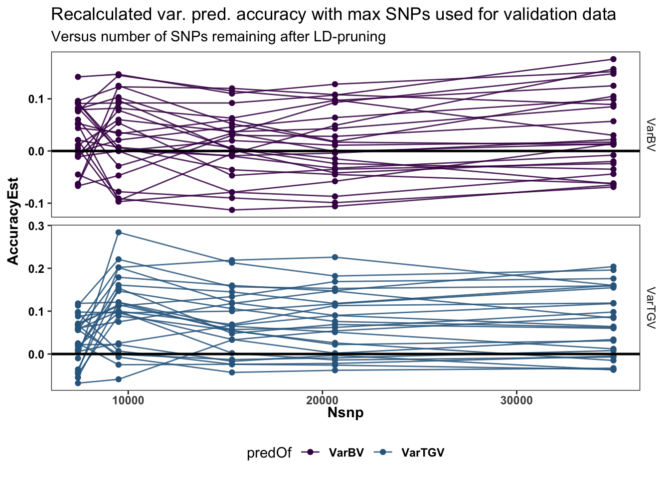
recalculated_accuracy %>%
    ggplot(.,aes(x=predOf,y=AccuracyEst,fill=predOf)) +
 ggdist::stat_halfeye(adjust=0.5,.width = 0,fill='gray',width=0.75) +
  geom_boxplot(width=0.12,notch = TRUE) +
  ggdist::stat_dots(side = "left",justification = 1.1,dotsize=0.6)+
  theme_bw() +
  scale_fill_manual(values = viridis::viridis(4)[1:2]) +
  scale_color_manual(values = viridis::viridis(4)[1:2]) +
  geom_hline(yintercept=0, color='black', size=0.9) +
  plottheme + theme(axis.text.x = element_text(face='bold'),
                    axis.title.x = element_text(face='bold')) +
  facet_grid(.~Nsnp,scales = 'free') +
  labs(title="Recalculated var. pred. accuracy with max SNPs used for validation data",
subtitle="Versus number of SNPs remaining after LD-pruning") 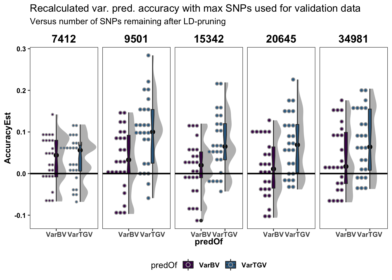
The above two plots (line plot and boxplots) show that:
- After re-calculating accuracy against the full SNP set, the lowest level Nsnp=7412 is indeed significantly worse in agreement with the standard cross-validation and the parent-wise CV cross-mean accuracy estimate.
- Reduced SNP density actually seems to stable or even slightly improved variance prediction accuracy
Time savings: 20K to 15K = 67%, 15K to 9.5K = 73% (49% over 20K)….not sure the 34 hrs for the original 34K markers is fair. I think the code in that run did not use multi-thread BLAS for variance prediction.
Last plot below just shows the re-calculated accuracy of CrossMean predictions, reinforcing that reduced SNP numbers provide stable predictions until the lowest level.
forplotmeans<-accuracy %>%
  filter(CVtype=="ParentwiseCV") %>%
  select(CVtype,Filter,results) %>%
  mutate(results=map(results,~.$meanPredAccuracy %>%
                       filter(Trait=="SELIND") %>%
                       select(Repeat,Fold,predOf,predVSobs) %>%
                       unnest(predVSobs))) %>%
  left_join(tribble(~Filter,~Nsnp,~ParentwiseRuntime,
        "50snp_25snp_pt98",34981,34.5,
        "1Mb_50kb_pt9",20645,10.65,
        "1Mb_50kb_pt8",15342,7.14,
        "1Mb_50kb_pt6",9501,5.28,
        "1Mb_50kb_pt5",7412,4.42)) %>%
  unnest(results) %>%
  mutate(predOf=factor(predOf,levels=c("MeanBV","MeanTGV")))
forplotmeans %>%
select(-obsMean,-ParentwiseRuntime) %>%
left_join(forplotmeans %>%
filter(Filter=="50snp_25snp_pt98") %>%
select(-predMean,-Nsnp,-ParentwiseRuntime,-Filter)) %>%
nest(predVSobs=c(sireID,damID,predMean,obsMean,famSize)) %>%
mutate(AccuracyEst=map_dbl(predVSobs,function(predVSobs){
out<-psych::cor.wt(predVSobs[,c("predMean","obsMean")],
w = predVSobs$famSize) %$% r[1,2] %>%
round(.,3)
return(out) })) %>%
select(-predVSobs) %>%
ggplot(.,aes(x=Nsnp,y=AccuracyEst,color=predOf,group=paste0(Repeat,"_",Fold,"_",predOf))) +
geom_point() + geom_line(alpha=0.85) +
theme_bw() +
scale_color_manual(values = viridis::viridis(4)[1:2]) +
geom_hline(yintercept=0, color='black', size=0.9) +
plottheme + theme(axis.text.x = element_text(face='bold'),
axis.title.x = element_text(face='bold')) +
facet_grid(predOf~.,scales = 'free') +
labs(title="Recalculated mean pred. accuracy with max SNPs used for validation data",
subtitle="Versus number of SNPs remaining after LD-pruning") 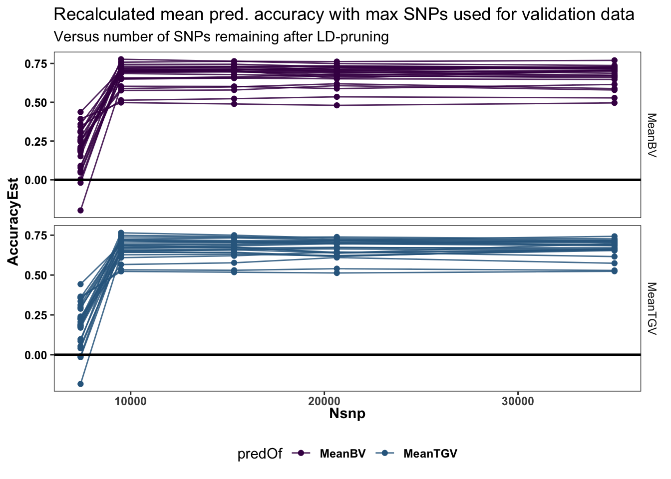
Recommendation:
Based on the above examination of the accuracy using reduced SNP sets, I propose the following practical procedure:
Fit genomic prediction models (
runGenomicPredictions()) with both the “full” SNP dataset (full_set) and an LD-prunned dataset (prunned_set) using at maximum “1Mb_50kb_pt6” (plink1.9 --indep-pairwise 1000 'kb' 50 0.6).[OPTION TO EVAL REDUCED SET BASED ON STANDARD CV ONLY] Conduct standard and parent-wise cross-validation with both sets
Predict cross means using full_set and prunned_set. Check their correlation. If suitable, proceed with variance prediction using the prunned_set.
Using chosen snp set, predict cross variances
Select crosses based on the full_set mean and (if relevant) the prunned_set variances to construct the cross usefulness criterion.
[FUTURE] Compare PHG-to-Beagle data
[TO DO] PCA
[TO DO] Compare kinships
[TO DO] Prediction accuracy - PHG
[TO DO] Compare PHG-to-Beagle accuracy
sessionInfo()R version 4.1.0 (2021-05-18)
Platform: x86_64-apple-darwin17.0 (64-bit)
Running under: macOS Big Sur 10.16
Matrix products: default
BLAS: /Library/Frameworks/R.framework/Versions/4.1/Resources/lib/libRblas.dylib
LAPACK: /Library/Frameworks/R.framework/Versions/4.1/Resources/lib/libRlapack.dylib
locale:
[1] en_US.UTF-8/en_US.UTF-8/en_US.UTF-8/C/en_US.UTF-8/en_US.UTF-8
attached base packages:
[1] stats graphics grDevices utils datasets methods base
other attached packages:
[1] ggdist_3.0.0 ragg_1.1.3 magrittr_2.0.1 forcats_0.5.1
[5] stringr_1.4.0 dplyr_1.0.7 purrr_0.3.4 readr_2.0.0
[9] tidyr_1.1.3 tibble_3.1.3 ggplot2_3.3.5 tidyverse_1.3.1
[13] workflowr_1.6.2
loaded via a namespace (and not attached):
[1] nlme_3.1-152 fs_1.5.0 lubridate_1.7.10
[4] httr_1.4.2 rprojroot_2.0.2 tools_4.1.0
[7] backports_1.2.1 bslib_0.2.5.1 utf8_1.2.2
[10] R6_2.5.0 DBI_1.1.1 mgcv_1.8-36
[13] colorspace_2.0-2 withr_2.4.2 mnormt_2.0.2
[16] tidyselect_1.1.1 gridExtra_2.3 compiler_4.1.0
[19] git2r_0.28.0 textshaping_0.3.5 cli_3.0.1
[22] rvest_1.0.1 xml2_1.3.2 labeling_0.4.2
[25] sass_0.4.0 scales_1.1.1 psych_2.1.6
[28] systemfonts_1.0.2 digest_0.6.27 rmarkdown_2.9
[31] pkgconfig_2.0.3 htmltools_0.5.1.1 dbplyr_2.1.1
[34] highr_0.9 rlang_0.4.11 readxl_1.3.1
[37] rstudioapi_0.13 jquerylib_0.1.4 farver_2.1.0
[40] generics_0.1.0 jsonlite_1.7.2 distributional_0.2.2
[43] Matrix_1.3-4 Rcpp_1.0.7 munsell_0.5.0
[46] fansi_0.5.0 viridis_0.6.1 lifecycle_1.0.0
[49] stringi_1.7.3 whisker_0.4 yaml_2.2.1
[52] grid_4.1.0 parallel_4.1.0 promises_1.2.0.1
[55] crayon_1.4.1 lattice_0.20-44 haven_2.4.1
[58] splines_4.1.0 hms_1.1.0 tmvnsim_1.0-2
[61] knitr_1.33 pillar_1.6.2 reprex_2.0.0
[64] glue_1.4.2 evaluate_0.14 modelr_0.1.8
[67] vctrs_0.3.8 tzdb_0.1.2 httpuv_1.6.1
[70] cellranger_1.1.0 gtable_0.3.0 assertthat_0.2.1
[73] xfun_0.24 broom_0.7.9 later_1.2.0
[76] viridisLite_0.4.0 ellipsis_0.3.2 here_1.0.1